
Innov Clin Neurosci. 2026;23(4–6):18–36.
by Shilpa Bajaj, MCA; Manju Bala, PhD; and Mohit Angurala, PhD
Dr. Bajaj is with Applied Sciences (Computer Applications), I.K. Gujral Punjab Technical University, Kapurthala, Punjab, India. Dr. Bala is with Department of Computer Science and Engineering, Khalsa College of Engineering and Technology, Amritsar, Punjab, India. Dr. Angurala is with Department of Computer Science, Guru Nanak Dev University College, Pathankot, Punjab, India.
FUNDING: No funding was provided for this article.
DISCLOSURES: The authors have no relevant conflicts of interest.
Abstract: To identify strokes, which rank among the leading global causes of death, doctors commonly employ computed tomography (CT) imaging. Researchers are increasingly applying deep learning (DL) and machine learning (ML) methods to improve the accuracy of stroke classification and detection. In particular, DL methods have demonstrated significant potential in segmenting stroke regions within brain medical images. However, training convolutional neural networks from scratch is challenging due to dataset size constraints. Achieving timely and precise stroke diagnosis remains a significant hurdle. The purpose of this research is to classify brain stroke cases using CT scan images through transfer learning strategies. Pretrained architectures including ResNet, VGG, Inception, and EfficientNet are utilized, with optimization carried out in the fastai framework to improve computational efficiency and reduce training time. We developed these artifical intelligence (AI) systems by training them with data, making adjustments throughout the process to ultimately categorize patients as having a stroke or not. We evaluated different models using measures such as accuracy, speed, and how well they differentiate normal and stroke-affected CT scans of the brain. This helped us choose the most effective model. In this research, ResNet50 outperformed other models in accuracy (88%), and DCNN was the most time-efficient model.
Keywords: Stroke, CT image classification, convolutional neural networks, deep learning, feature extraction
Introduction
A sudden interruption of blood flow to the brain triggers a stroke, a medical emergency requiring immediate attention.1 A lot of brain cells could die because of this, which could lead to problems like paralysis, speech problems, and vision problems. Early diagnosis and treatment are very important for limiting damage and making things better for patients. It is important to note that ischemic stroke is a heterogeneous condition, and the evolution of an ischemic lesion can differ greatly among patients. Factors such as collateral circulation, reperfusion timing, and individual biological responses influence the rate and extent of tissue damage, making lesion progression highly variable. This heterogeneity complicates timely diagnosis and prognosis, further emphasizing the need for advanced computational methods that can adapt to diverse clinical presentations. Computed tomography (CT) scans help doctors evaluate and diagnose stroke patients because they show information about the brain’s structure. However, it may be difficult to accurately identify and differentiate a stroke spot on a CT scan. The capability to identify an ischemic lesion on noncontrast CT is influenced by multiple factors, including the size and anatomical location of the lesion, the underlying cause, and even the availability of supporting clinical information. Radiologists often rely on a neuroanatomical hypothesis to guide their interpretation, rather than depending solely on image contrast. This highlights both the challenge and importance of integrating computational tools that can support lesion recognition under such complex conditions. Due to the complexity of the pathology and the small magnitude of the signs of complications from a stroke, existing image analysis techniques cannot adequately explain the variety of seizure symptom patterns on the brain. Several technologies have been applied to detect brain strokes in CT scans to discriminate them from other forms of damage. Medical imaging is urgently needed for prompt and precise diagnosis, especially for neurological disorders like stroke. However, current techniques also often encounter problems in efficiently processing and analyzing the massive amount of medical images. As a result, the diagnosis may be postponed, negatively affecting the patient. Through the implementation of advanced methodologies, such as fastai, which simplifies deep learning (DL) model development and deployment,2–5 the challenges can be overcome to provide faster and more accurate diagnosis of stroke. This allows for enhanced image contrast, extraction of the most relevant features, and, subsequently, application of transfer learning models. DL algorithms display high-level results in various image designations, including the brain infarcts identification. One study by Gao et al6 created a way to group CT brain images using DL. First, they used a dataset to teach DL networks. Then, they tested how well they could group different brain diseases using CT scan data. The study employs hybrid convolutional neural network (CNN) architecture and an advanced hand-crafted method with the objective of classifying CT brain images into Alzheimer’s disease (AD), lesion, and normal aging categories. Kuo et al2 used a large dataset to train their hybrid CNN-based classification model and demonstrated accurate classification performance at finding and locating hemorrhages. This could help doctors find people who have had a brain bleed quickly and help them. The study utilizes a fully CNN.7 In studies reported by references 7 and 8, fully CNN were utilized for automated brain image classification trained on head CT scans to detect acute intracranial hemorrhage, demonstrating performance exceeding that of radiologists. While the performance of the 2 studies is commendable, they did not employ transfer learning or fastai techniques in their methodologies. In addition to the architecture, various data characteristics significantly impact the training of a transformer model. A dataset6 of 285 CT brain images were categorized into Alzheimer’s disease, lesion, and normal aging classes. Given the study’s small dataset, transfer learning techniques could be employed to mitigate this limitation. A study by Gautam et al9 combines CNN, Vision Transformers (ViT), and AutoML for stroke classification with CT scans, improving diagnostic accuracy and easing radiologist workload. VGG-16, VGG-19, ResNet50, and ViT were individually assessed for slice-level predictions, without leveraging fastai techniques. While existing literature extensively explores DL6,10 techniques for classification, there is a notable absence of integration with the fastai library, limiting both efficiency and accuracy. Furthermore, the prevalent use of small datasets11 in these studies hinders robust model development. Additionally, while machine learning (ML)12–14 techniques are frequently applied in medical imaging for various diseases, the focus on brain infarction remains limited.15–19 To address these gaps, this research aims to enhance the accuracy and speed of brain infarction classification based on transfer learning20 and integrating fastai21 techniques. Through these efforts, the study seeks to achieve greater efficiency and a reliable framework for diagnosis, thereby addressing critical needs in clinical practice. This research examines how DL can be used to improve the diagnosis of brain strokes. To train our DL models, we employed switch learning techniques within the fastai DL framework. Transfer learning speeds up the process of making models by using weights that have already been learned. The process of learning traits from different types of data also helps improve model performance. Fastai makes it possible for ML models to give more accurate and timely results by simplifying the training process. Generalizing DL models22–24 for stroke detection across diverse datasets is a challenge. We can make DL models quickly and well with the help of fastai and transfer learning.
The key contributions of this study are outlined as follows:
- A novel preprocessing pipeline combining segmentation-based methods was applied to increase image contrast, thereby supporting improved brain infarct diagnosis.
- CT images were preprocessed and standardized to correct inconsistencies and improve quality.
- The images were transformed into binary matrices, after which a feature selection model was employed to extract the essential aspects.
- Transfer learning models, such as VGG-16, ResNet50, Inception v3 and DCNN, were utilized within the fastai framework to enable efficient and accurate brain infarct detection.
- Finally, a performance comparison of these models was conducted, accompanied by an assessment of their advantages and disadvantages.
First, we provide an introduction to brain stroke and review a wide range of studies on utilizing transfer learning for medical image interpretation, with a specific focus on detecting brain infarcts. Then, we go into detail about the data and methods that were used to classify strokes. Next, there was a thorough look at how well the models performed classification. The classification results and their clinical significance are evaluated and discussed. Finally, we briefly talk about the main findings and possible future research paths.
Literature survey
We conducted a literature review to look into the studies on useful models that are currently used to quickly group brain infarcts into different groups. A thorough study of how ML techniques can be used to help people who have had a brain stroke was done by Sirsat et al.1 They talked about the pros, cons, and uses of ML in identifying and finding strokes while looking at a number of studies. The review synthesized existing research in the field and identified promising avenues for future inquiry.
Gao et al6 created a way to group CT brain images using DL. First, they used a dataset to teach DL networks. Then, they tested how well they could group different brain diseases using CT scan data.
Li et al10 built a model and tested how well it could find and group blood spots. It was done so that doctors could find and treat people with brain bleeds more quickly.
Khan et al4 dreviewed recent machine ML and DL approaches for detecting 4 major brain diseases: Alzheimer’s disease, brain tumor, epilepsy, and Parkinson’s disease. They analyzed 147 research articles, discussed commonly used datasets and feature extraction techniques, and compared different AI-based diagnostic methods. The study also summarized key findings and highlighted major challenges and future directions in AI-based brain disease diagnosis.
A large dataset was used by Kuo et al2 to teach the system and show that it was good at locating hemorrhages. This could help doctors quickly identify patients who have had a brain bleed.
A CNN-DL technique was applied by Chin et al3 to construct a ML model for early ischemic stroke detection. They taught the program how to correctly recognize the first signs of an ischemic stroke by using data that was relevant, which might help facilitate a quicker response.
In their study, Khan et al4 proposed a DL model for identifying and delineating bleeding tumors in brain CT scans. With the help of DL methods, they made a model that could correctly find and split CT scan area of blood. This would help doctors find and treat people who have brain hemorrhages.
In their article, Dourado et al5 described an open DL framework for online medical picture recognition that is based on the Internet of Health Things (IoHT). Interoperability and linking of IoHT devices make it possible for DL algorithms to be used for real-time medical picture recognition through the framework. The goal of the plan is to make medical picture analysis faster and easier to access, so that diagnoses can be made quickly and correctly.
In their study, Liu et al11 proposed a combined ML framework for stroke prediction based on medical datasets with class imbalance. Because the data were not all the same, they used different ML methods, including undersampling and oversampling, to make the model better at predicting strokes. The method tries to make better guesses about brain strokes, even though the data are not all in one place. This might help clinicians catch strokes early and stop them.
A DL Internet of Things (IoT) system for rapid stroke detection in head CT images was introduced by Dourado Jr. et al.25 IoT gadgets and DL are used by the system to find and spot strokes right away. The IoT gadgets are used in this way to use DL models that help doctors find a stroke early and properly. This would allow them to move quickly, potentially helping the patient do better.
Karthik et al26 used a fully convolutional network (FCN) to make a deep-trained method for sorting ischemic lesions from different types of magnetic resonance imaigng (MRI) data. They used a set of multimodal MRI scans to make the FCN model, which correctly separates ischemic regions and helps doctors diagnose and plan treatment for people who have had an ischemic stroke by combining different imaging types.
He et al27 were the first to describe deep residual learning, a new type of neural network design that uses leftover connections to make training of very deep networks more efficient. Their technique significantly improved photo recognition accuracy, which made it simpler to train previously challenging deep models. This innovation is currently a major component of modern CNN design.
In their article, Howard et al28 proposed MobileNets, a series of CNNs optimized for resource-constrained environments, such as mobile and embedded devices. Because they need a significant reduction in parameters and processing resources to achieve the same level of performance, these networks perform very well in real-time and resource-constrained applications. A key part of mobile artificial intelligence (AI) is the Mobile Nets design, which lets devices with limited computer power do a variety of visual tasks.
Simonyan and Zisserman29 came up with the idea of extremely deep convolutional networks, which made a big step forward in the field of large-scale picture recognition. This important finding has greatly helped the fields of DL and picture analysis.
To find out the carotid artery intima-media thickness using ultrasound images, Savas et al30 compared different DL models. The authors proposed a new DL architecture, CAIMTUSNet, and demonstarted that it performed better than existing models for medical image analysis, therby supporting improved cardiovascular health assessment.
DenseNet, a new neural network design enhancing both efficiency and classification performance in DL for computer vision, was proposed by Huang et al.31 There are tight and efficient links between each layer and every other layer, which helps gradient flow and feature reuse. This approach improved both the usability and cost-effectiveness of DL architectures in computer vision. It also helped the models perform better on tests of grouping pictures.
Proposed by Chollet,32 this Xception architecture employs depth-wise separable convolutions to enhance the learning capability of deep neural networks. With this method, you can quickly and easily describe the links between space and channels. Xception did better at several computer vision tasks, which shows how important it is for DL projects to use efficient convolutions.
In their work, Szegedy et al33 presented Inception-v4, an updated iteration of the Inception CNN designed for improved performance. The study came up with new design ideas and parts that would make feature extraction and network depth more efficient. Their work moved the field of computer vision forward by making CNN work better and helping with jobs like identifying and sorting photos.
Kingma et al34 advanced the field of DL by proposing a technique that enables more effective learning of neural network representations. New research in neural networks and representation learning is often shown at the International Conference on Learning Representations. Alhatem and Savaş investigated the use of transfer learning for classifying stroke using various computer science techniques.20 They discussed using models that had already been trained to make stroke classification more accurate and helped come up with better ways to use medical images to diagnose strokes.
An extensive investigation of medical image segmentation and feature extraction was presented by Chowdhary and Acharjya.7 They talked about the newest findings and changes that have happened in this area.
Zhang et al8 created a CNN method that can be understood and that changes the model itself in real time to correctly group different types of ischemic strokes.
Salau and Jain35 conducted a comprehensive study on feature extraction methods, detailing the various types, techniques, and their applications.
To improve the accuracy of identifying different types of ischemic strokes while keeping model interpretability, Fan et al36 used electronic health data to compare 6 ML models for predicting arterial atherosclerosis in people who do not have any symptoms.
Ortiz-Ramón et al37 investigated the use of texture analysis in brain MRI scans to identify ischemic stroke lesions. Researchers have made strides in finding these defects and understanding how strokes change the brain. This has big effects on how they treat stroke patients. Han et al38 came up with a new way to classify ischemic stroke subtypes that includes the reasons and treatments in order to make the classification more accurate. Goldstein et al12 applied the Trial of ORG 10172 in Acute Stroke Treatment guidelines to enhance the accuracy of stroke subtype classification. As a result, strokes were put into more accurate groups. Sung, Lin, and Hu13 used text mining and supervised ML to create a methodology for ischemic stroke phenotyping utilizing electronic medical records (EMRs). Govindarajan et al14 made a classification method for stroke sickness that is based on ML, which makes the diagnosis more accurate. Walsh15 reviewed the current state and future of noninvasive monitor devices for finding strokes before patients get to the hospital. The study discussed the technology’s future possibilities and gave an overview of how it works now. Salucci, Polo, and Vrba16 came up with a new learning-by-examples method that can be used to invert microwave scattering data from patients with stroke in real time. Using advanced signal processing techniques, this method makes it easier to understand the data and could lead to better stroke identification. Bajaj et al17 conducted an evaluation of 3 ML models for stroke detection, comprising OzNet-mRMR-NB, Logistic Regression, and an Ensemble CNN, based on medical imaging datasets. They developed the Ensemble CNN by combining ResNet and VGG19, achieving the highest accuracy (92.43%) and strong performance metrics. The study demonstrates that integrating multiple CNN architectures improves prediction accuracy and has potential for clinical application in timely stroke diagnosis.
There are many different topics that are related to neural networks and DL uses. An online guide called Neural Networks and DL, written by Michael Nielsen,18 provides information about neural network concepts and DL methods. Pedregosa et al19 developed Scikit-learn, a widely used Python library that offers a versatile toolkit for applying various ML algorithms. Due to their work, ML methods are now much easier to find and use in the Python computer community. Fastai is a high-level API that was created by Jeremy Howard and Sylvain Gugger21 to make it easier for developers to make and train DL models. Neural Networks: Tricks of the Trade, written by Orr and Müller,39 is a great resource for people who work with neural networks. This collection gives methods and points of view that help the field grow. Raj et al22 developed a way to group brain strokes into different groups, called StrokeViT. They used automatic ML and vision transforms in their study to improve the accuracy of stroke classifications. Gautam and Raman9 came up with a way to correctly separate brain hemorrhagic and ischemic strokes that used CNN. Their study uses cutting-edge ways to improve how strokes are grouped. Karthik et al23 looked at the newest advances in MRI and DL and how they might be used to diagnose brain strokes. Their study shows how DL methods might be combined with advanced image techniques to make better plans for finding strokes. Wang et al40 discussed how ML has changed the way medical imaging is done. Their study shows that ML methods are being used more and more with picture restoration techniques. HiResCAM, a way to describe CNN’s decisions, was created by Draelos and Carin.41 HiResCAM is a good alternative to Grad-CAM, which is often used to explain CNN’s decisions. HiResCAM is better than Grad-CAM in many ways, such as being more accurate and easier to understand. Research was done by Magadza and Viriri42 shows he most recent progress on how to use DL methods to group brain tumors. Folego et al43 made the suggestion of using a whole-brain 3D-CNN MRI to find AD. By mixing cutting-edge imaging techniques with DL, their method makes it easier to diagnose AD. Haller et al44 introduced the RADIOLOGY checklist, a valuable tool for assessing the clinical application of AI technologies in neuroradiology. In this area, the checklist rates the value and healing importance of AI apps. RadImageNet is a large open-source database of medical images created by Mei et al45 that can be used for radiology transfer learning. RadiImageNet is a very useful tool for making and testing DL models for different radiology uses. Bajaj et al46 applied and categorized data augmentation techniques on brain CT images to expand the training dataset and improve deep learning model performance. They evaluated 4 augmentation levels—absent, basic, intermediate, and advanced—to determine which approach enhances accuracy and robustness. The study aimed to identify the most effective augmentation strategy for reliable brain stroke detection, with the goal of making transfer learning in medical image processing more effective and efficient. Wang et al47 developed a novel federated semi-supervised learning (FSSL) framework utilizing data from 6 centers to enhance lung tumor segmentation performance. They introduced a dynamically updated algorithm for model parameter aggregation, leveraging both the quality and quantity of client data. Additionally, they explored the FAIR data principle to increase data accessibility in the federated learning network, leading to improved segmentation results compared to traditional DL and recent FSSL methods. Pérez-Velasco et al48 used DL and explainable AI to understand the brain mechanisms behind motor imagery. They found that focusing on a broader brain activation network improved decoding accuracy. By applying SHAP to electroencephalogram data, they identified the involvement of multiple brain regions beyond M1 and S1, leading to better electrode configuration for high brain-computer interdace (BCI) accuracy. Farkhani et al49 evaluated DL segmentation tools, including a novel volumetric segmentation model with self-attention, on FLAIR MRI data from the LISA project. They explored weighted loss functions and ensemble models, achieving high segmentation performance comparable to expert raters, and validated their approach on an independent dataset from the MICCAI WMH challenge, demonstrating superior generalizability. Lo et al50 developed a deep CNN (DCNN) model for automatic identification of acute ischemic stroke using noncontrast CT (NCCT) images. They trained a program (ResNet18) on 2,400 brain scans, using prior information from general images for high accuracy. They also compared program designs and data augmentation, achieving 90% accuracy, demonstrating DL’s efficacy in stroke diagnosis. Abbaoui et al51 completely investigated DL models for precisely arranging ischemic strokes utilizing clinical information from Morocco. They used the OSEMN approach and transfer learning with VGG-16, achieving a remarkable validation accuracy of 90%, outperforming other state-of-the-art models like ResNet50, Inception v3, and VGG-19. Their discoveries feature the viability of VGG-16 and stress the significance of choosing reasonable models for clinical imaging undertakings, displaying the capability of trend setting innovations in working on analytic exactness and medical care results.
The review provides insight on how to make cerebrum stroke classification models that function accurately. Studies show that these models can be used to find, evaluate, and treat strokes. There are still problems regarding unequal data, ethics, and making quick diagnoses, even though these models can have the ability to improve patient results. These problems need to be fixed so that these methods can be used more in medical picture analysis. We found that the fact that many models were trained on small datasets made their learning curves longer. To solve these problems, we used transfer learning methods along with the fastai package. Fastai is a DL library that facilitates the training and deployment of ML models. Through the use of transfer learning, we can train a new model on a smaller dataset using a pretrained model as a starting point. Our training methods help our models learn and perform better than traditional methods.
Research gaps. Many studies in the literature review employ DL techniques but lack integration with the fastai library. The majority of studies utilize small datasets, posing a limitation to the research. ML techniques are predominantly applied in studies focusing on different diseases. Traditional methods contribute to slower performance across various studies.
Objectives. We aimed to improve the accuracy and adequacy of brain infarct classification through the incorporation of transfer learning and fastai techniques. In this technique, we incorporate various significant changes. To improve brain infarct classification exactness and dependability and make analyses more exact, we set progressed ML procedures into practice. Second, we aimed to accelerate the categorization process so clinical experts can assess patients more rapidly, which prompts improved patient care. Third, transfer learning was utilized to get benefits from recently trained models, further developing proficiency and versatility, particularly in circumstances where data were restricted. Lastly, to work on the general adequacy of our DL system, we included the fastai library, which is known for its adaptability and speed, to streamline the model building, training, and evaluation procedures.
Methodology
In this research, we used the fastai library to quickly and accurately classify strokes from brain CT images.
Dataset compilation. To train and evaluate our model, a large number of brain stroke CT scan images were required. For this purpose, we utilized the Brain Stroke CT Image Dataset, available on Kaggle, a widely used online platform for data science resources. This dataset comprises CT images collected from multiple medical institutions, providing diverse samples for effective stroke detection. We use 2,250 images from this website (Figures 1 and 2). However, the dataset does not uniformly specify the time interval between symptom onset and CT acquisition. As a result, the images likely represent a mixture of acute and subacute ischemic stroke stages. Since lesion detectability on NCCT is strongly time dependent—with early ischemic changes being subtle and later changes more pronounced—this variability might have influenced both the ground truth labeling and the performance of our models.
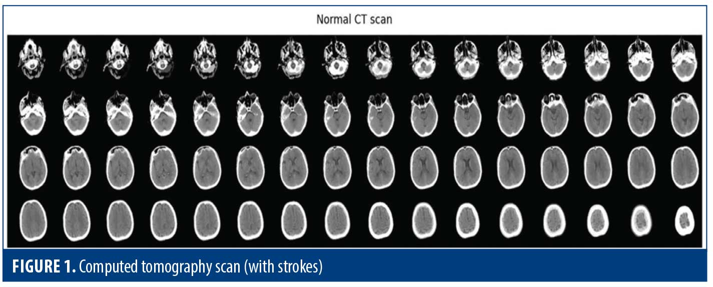
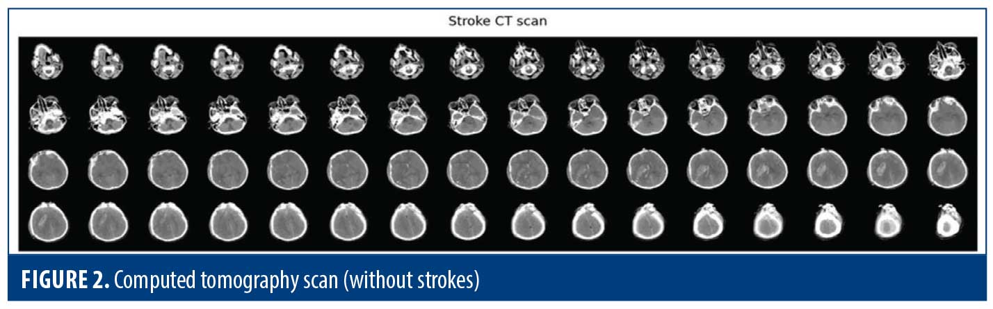
Image data preprocessing. Every image from the dataset went through the following important steps in our preprocessing pipeline. First, it resized an image to 224×224 pixels, since all images being the same resolution influences the stability of the model. Next, it converted each image into an RGB color space. This kept the color representation of all images uniform and helped the model learn the visual features in each image effectively. Finally, the preprocessed images were converted to NumPy arrays. These arrays hold the values of pixel intensity for each image, thus working with our model in training and evaluation task. The data were then ready to go into the model for more in-depth analysis and classification after the completion of this step.
Class labels. Having added the class names to our dataset, we started by making 2 records, normal_label and stroke_label. For the normal_label, we set each component to 0, which demonstrates the normal class. Then for the stroke_label, we set each component to 1, demonstrating the stroke range. We merged these components with the + operator to make a single list named target_label. This accumulated list contained the class names of all pictures in our dataset, where normal pictures are addressed by the mark 0 and stroke pictures by the name 1. Finally, we printed the length of the target_label list. It distinguished the total number of images in our dataset. This gave a total of 2,501 images.
Convert image data and target labels into array. Here, we converted our image data and labels into an interpretable format using the ML model. We had just converted our graphics into NumPy arrays, which is like numbers that a computer can understand. This way, we could retrieve the pixel values of each of the images and process them quickly. Similarly, we transformed the list of labels into a NumPy array. Each label in this list corresponded to the class of the corresponding image. These changes improved the process of training and testing our ML model, respectively, making it more efficient and simpler. After these steps, our data was ready for the next phase of analysis.
Preparation of training and testing sets. In this step, training and testing sets were created from the dataset. Train_test_split function was used to split our dataset. We allocated 10% of the dataset for testing to make sure that we had enough unseen data to evaluate our model’s performance. Setting Shuffle=True ensured that our data was randomly shuffled before splitting, reducing any bias in the dataset. After splitting, we checked the sizes of our training and testing datasets and printed out the results. This approach helped balance our training and testing datasets, facilitating effective training and testing of the model.
Scale the data. This was the step in which we prepared the image data for training the model. It allowed us to adjust the values of the pixels in the images. Each pixel was divided into 255 units, which is the maximum value a pixel can take. This scaling process was crucial to help the model effectively learn from the data. This increased the pixel values between 0 and 1 across all components to a similar scale, and it kept any single component from totally driving the learning process to help our model learn in a more accurate and efficient way. After scaling, both x_train_s and x_test_s had modified image data, ready for training. This scaling of the data allowed our model to exploit information from the image better, resulting in much better performance in terms of training and testing.
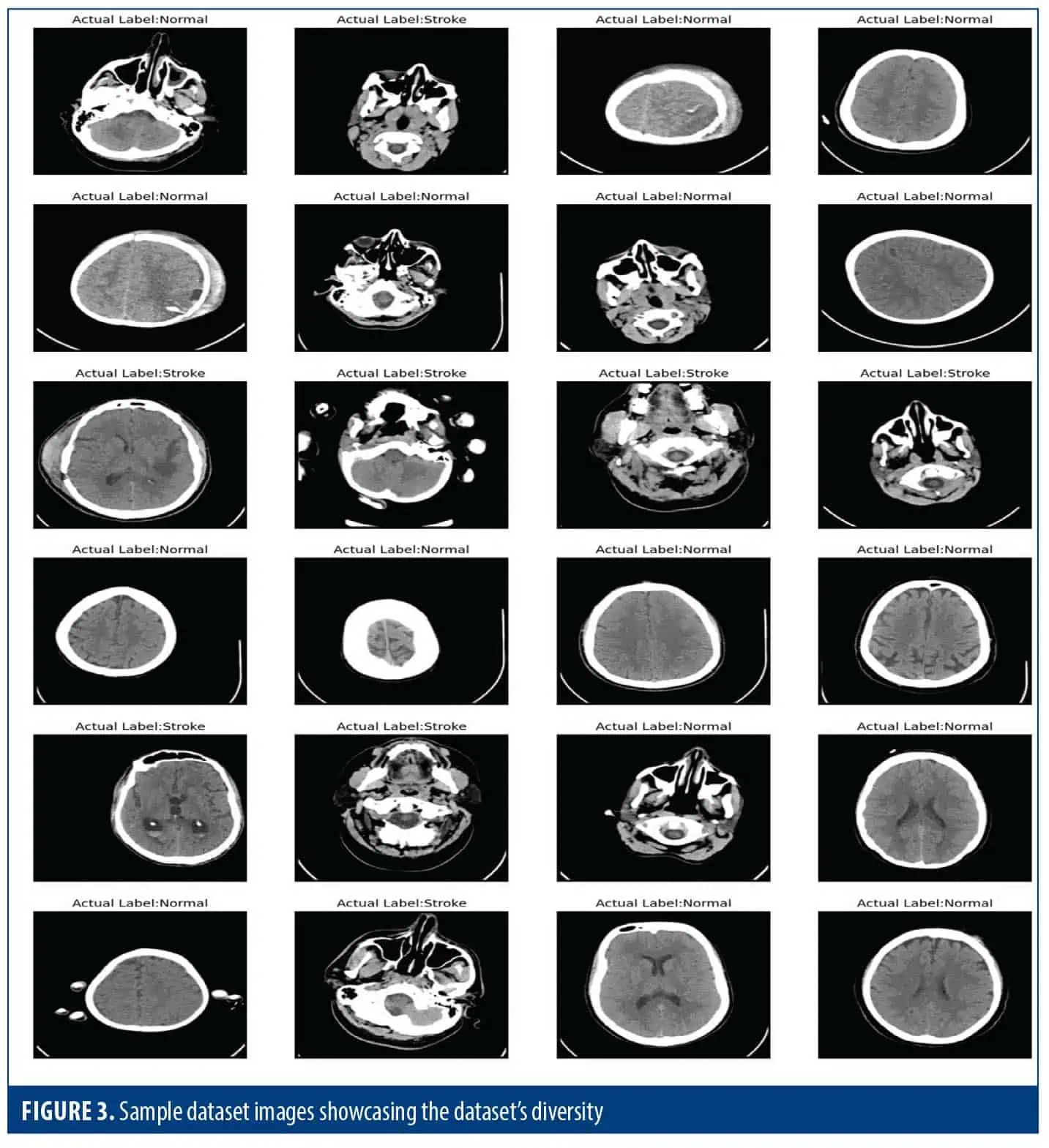
Image data visualization. In this part of our research, we plotted some samples from our dataset with their class labels. We first defined the class labels for 2 classes to be “Normal” and “Stroke” for the classes present in the dataset. Next, we set up a figure for the images and arrange them in a 6×4 grid within the figure. We then looped through the first 24 images in our training dataset (Figure 3).
Procedure. We utilized different versions of CNNs, including DCNN, VGG-16, ResNet50, and Inception v3, which have been trained on ImageNet, a comprehensive dataset containing millions of images. These models learned to recognize general features in images, which was helpful for tasks such as categorizing images. We applied these models to detect brain strokes as follows:
- Choose a dataset: First, we gathered a dataset containing images of brains, some with strokes and some without.
- Merge the images: We combined the images of brains with strokes and those without strokes into 1 dataset.
- Select pretrained models: We selected some pretrained CNN models, mentioned earlier.
- Train the models: Transfer learning technique was used, where we took the pretrained model and fine-tuned it on our dataset. We did this using the fastai library, which helped with DL tasks.
- Evaluate the performance: We used appropriate metrics to measure how well our model was doing at detecting strokes.
- Compare results: We repeated the process with other transfer learning techniques or different pretrained models to see which one performed best for our task.
Through these steps, we determined the optimal transfer learning approach for precise brain infarct classification, thereby enhancing stroke diagnosis and treatment outcomes. (Figure 4).
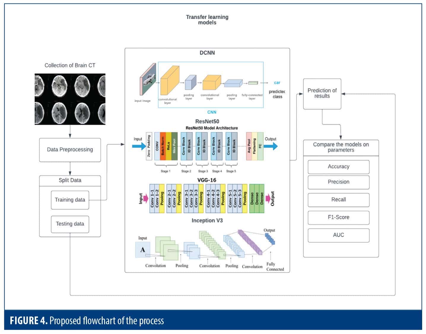
Overview of transfer learning techniques for medical imaging. This section focuses on transfer learning using CNNs pretrained on the ImageNet dataset, which contains 1.28 million images across 1,000 classification categories.ResNet5012 is one of these architectures. This model is a 50-layer deep neural network, intended to mitigate the vanishing gradient problem by incorporating shortcut connections. Because of its ability to capture very complex features, ResNet50 has been successful in a variety of computer vision applications, including image segmentation.
MobileNet-V213 is a CNN model designed to be computationally efficient while maintaining good accuracy. It does this by using skip connections and linear bottleneck blocks. MobileNet-V2 consists of 16 segments and is primarily used for tasks such as image classification because of its balance between computational cost and accuracy. Known for its winning performance in the 2014 ImageNet competition, the VGG-16 scheme14 relies on a coherent scheme of 3×3 convolutional filters at stride 1 and 2×2 max pooling layers at stride 2. This scheme has made VGG-16 a cornerstone model in computer vision.
EfficientNet15 goes beyond the traditional CNN algorithm by introducing a new way of thinking. This method measures all aspects of the mesh (depth, width, and shape) accurately with a single optimized multiplier. This approach enables EfficientNet to achieve high accuracy while maintaining its functionality, making it highly applicable to diverse computer vision applications. EfficientNet differs from standard ad-hoc scaling methods in that it uses set scaling factors to improve processing speed and efficiency, as well as to scale the mesh appropriately. Image labeling is a popular method, as it is used to solve problems because it can be scaled up or down.
DenseNet16 employs dense connectivity, in which every layer communicates directly with all other layers within a block, so that all preceding layers contribute to its input and its own feature maps are propagated forward to all following layers. Due to its densely connected design, it provides improvement, which encourages feature reuse, enhances gradient flow, and yields effective parameter utilization. DenseNet is very helpful for image categorization and other computer vision issues. Xception,17,18 which stands for extreme version of Inception, is a CNN architecture developed by Google. It has been proven to outperform Inception v3 on various computer vision tasks, including those using datasets like ImageNet, ILSVRC, and JFT. Xception stands out in image classification and feature extraction due to its use of a modified depthwise separable convolution. This technique efficiently captures intricate image details by performing computations more efficiently compared to standard convolutions.
In our research, we tested these models using data for detecting strokes in brain CT scans. All experiments were performed using a system equipped with 12 GB RAM and a Colab GPU. To implement the pretrained CNN models, we used the Keras package, and at the backend we use TensorFlow. Neural weights were updated throughout the training process using the Adam optimization approach, which was dependent on the training data.19 Ten epochs of training time and a batch size of 20 was used in training of models.
Evaluation metrics for binary classification models. Binary classification models that divide data into 2 classes are commonly assessed using several key metrics.
Loss: Measures the model’s performance during training based on the selected loss function.
True positives (TPs): Instance that are correctly predicted as positive.
False positives (FPs): Instances that are incorrectly predicted as positive.
True negative (TNs): Instances that are correctly predicted as negative.
False negatives (FNs): Instances that are incorrectly predicted as negative.
Accuracy: The proportion of correctly classified instances out of the total instances.
Precision: The proportion of correctly predicted positive instances out of all instances predicted as positive.
Recall: Indicates how effectively the model identifies all actual positive cases.
Area under the curve (AUC) of a receiver operating characteristic (ROC) curve: Summarizes the overall performance of a binary classification model. It represents the probability that the model ranks a randomly chosen positive instance higher than a randomly chosen negative instance.
AUC: Represents the total area under the ROC curve, summarizing the model’s ability to distinguish between classes.
True positive rate or sensitivity at threshold t [TPR(t)]: The proportion of actual positives correctly identified by the model at a given classification threshold.
Classification threshold (t): A value between 0 and 1 that determines the cutoff for classifying instances as positive or negative—0 means all instances are classified as negative, 1 means all are classified as positive.
Integral (∫): Denotes the summation of the area under the curve.
Experimental results
Assessment of model performance. We carefully looked at each model to find out how well it can make predictions,and evaluated measures such as F1 score, memory, and accuracy to show where each class is good and where it needs to improve. Using accuracy and weighted average F1 score, in addition to the F1 score, we provide a detailed evaluation of the model’s performance. This comprehensive analysis highlights not only the accuracy of the models but also their ability to distinguish and correctly classify instances across different classes.
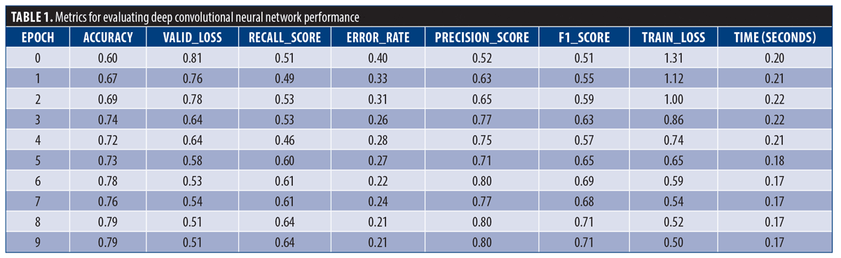
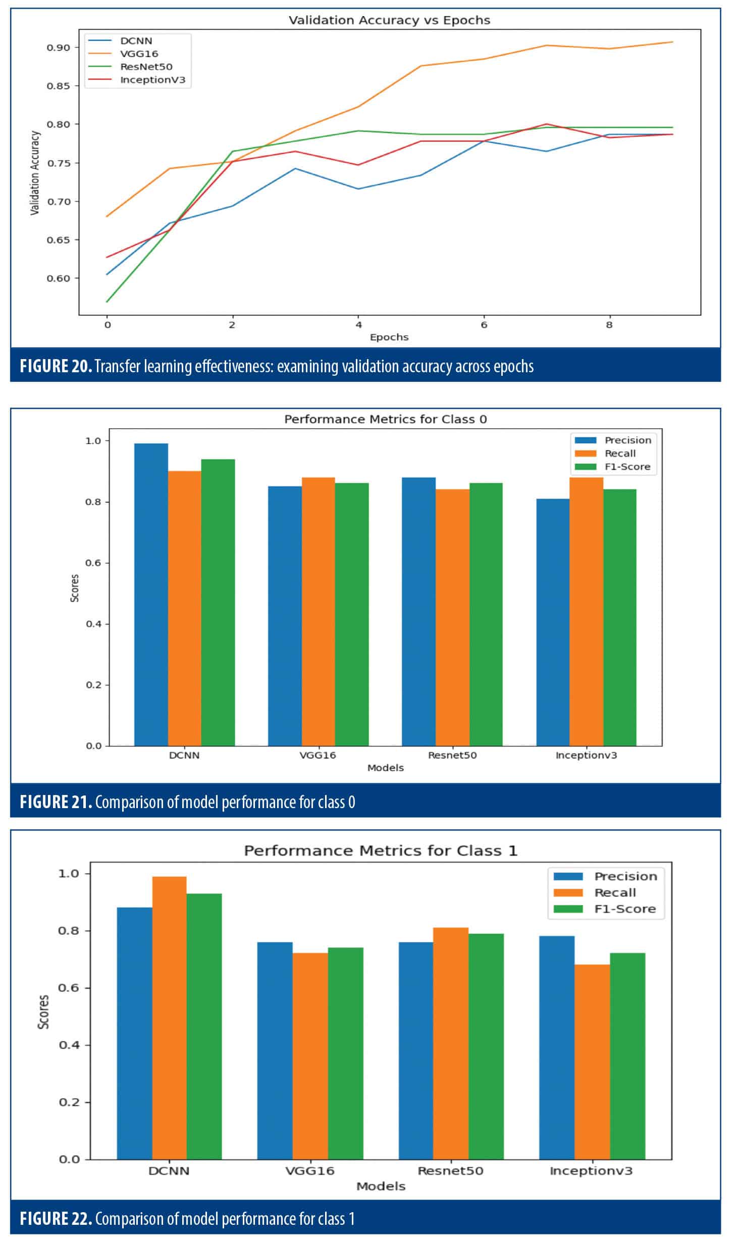
DCNN. In training, images were resized and batch transforms for diversity were applied. After 10 epochs, the model has a training loss of 0.50 and a validation loss of 0.51, indicating good fit and generalization. It achieved 78.67% accuracy on validation data but had a 21.33% error rate. The recall score was 64.13%, and the precision score was 79.73%. The F1score, representing balance, was 0.71. Each epoch took approximately 17 seconds (Table 1). These metrics give a snapshot of the model’s performance and improvement over training.
A visual examination of the model’s performance is shown in Figure 5. It allows us to check the classification accuracy of the model based on the comparison of the model’s predictions and the actual scores. In addition, the figures show the difficulty level of each forecast and give a hint about areas that can be optimized. In addition, the probability distribution of the model’s predictions gives the degree of confidence in the classification. This detailed visualization helps to assess the general model’s performance in terms of accuracy and predictiveness.
The grid format of the model’s predictions is displayed in Figure 6, beside the associated ground truth lines. This kind of visualization gives a fast and efficient way of measuring model performance under different conditions. Through analysis of the network, we can know the model’s capability in handling studies and its possible strengths or weaknesses; analysis of the network helps assess the model’s capability to handle various cases, identify its strength and weaknesses, validate its performance, and highlight areas for further improvement.
Figure 7 shows how well the model performed in putting the data into 2 groups via the confusion matrix. In class 0, there were 137 events, and 19 of these were incorrectly anticipated by the model as class 1 (FP), while 118 were accurately identified as class 0 (TN). In class 1 there were 88 samples, of which 25 samples were incorrectly identified as class 0 (FN) but 63 were correctly identified as class 1 (TP). This confusion matrix illustrates the model’s performance in detail, highlighting its accuracy in classifying samples and indicating its specific error.
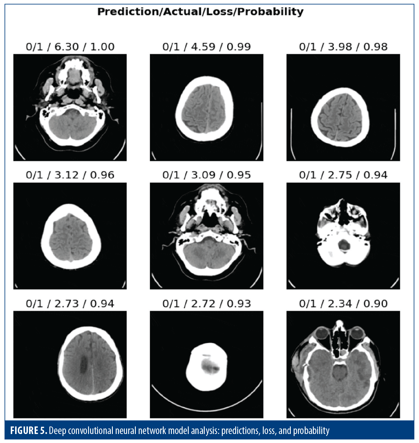
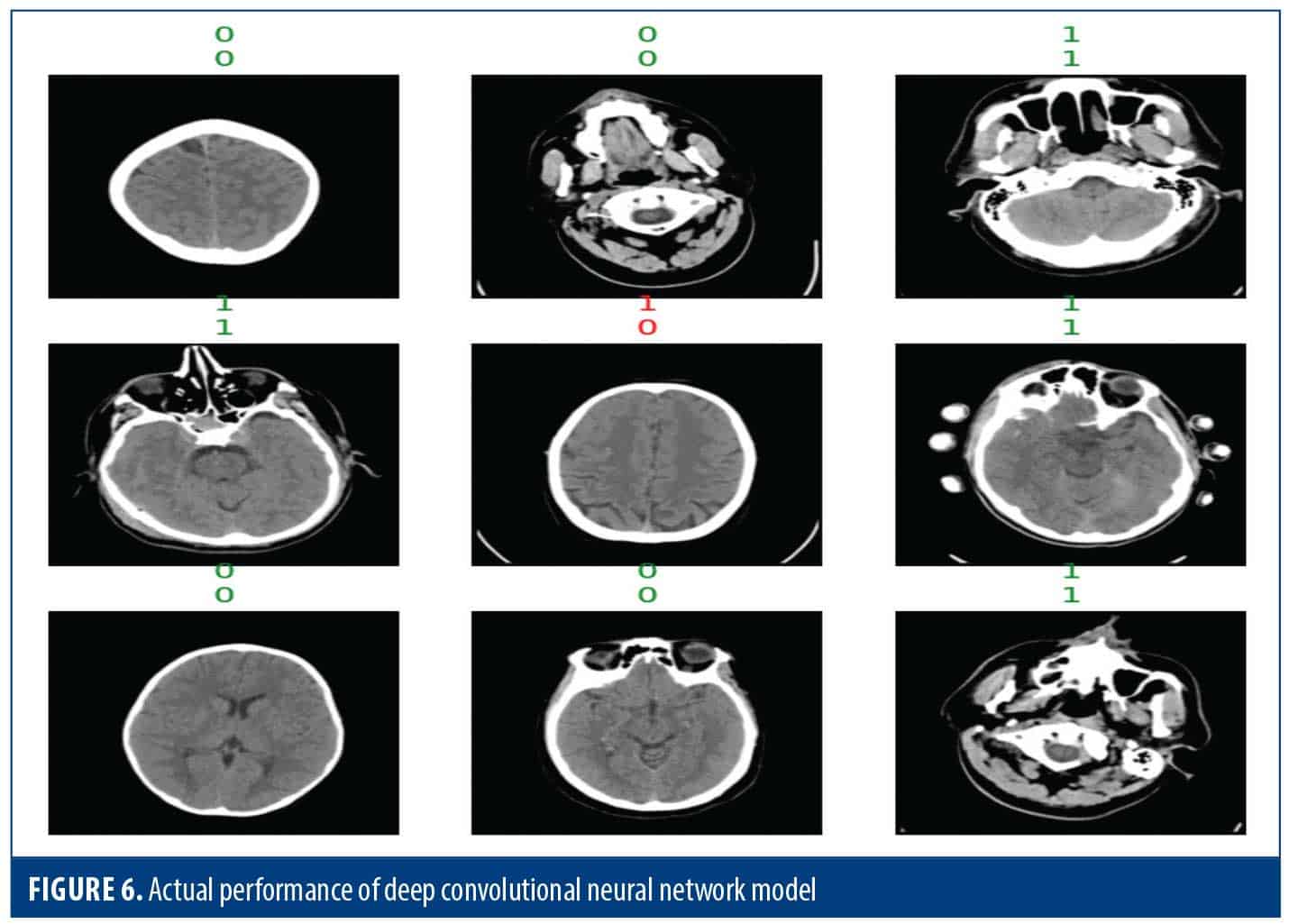
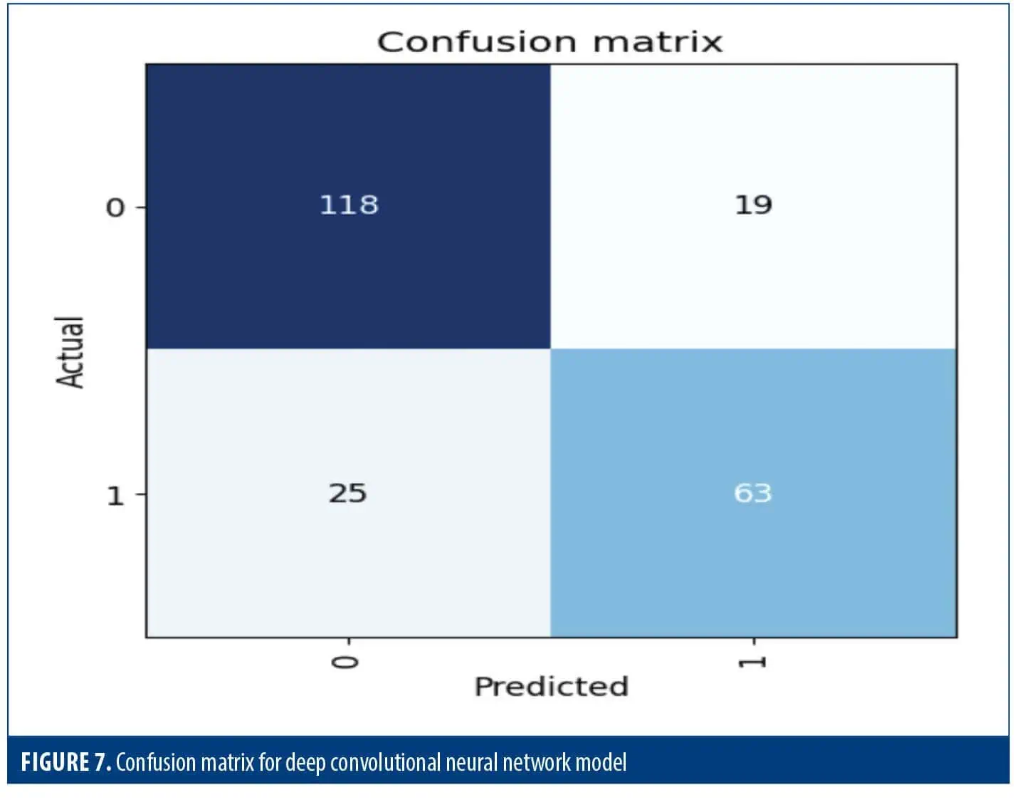
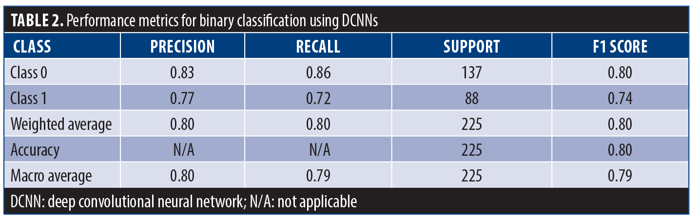
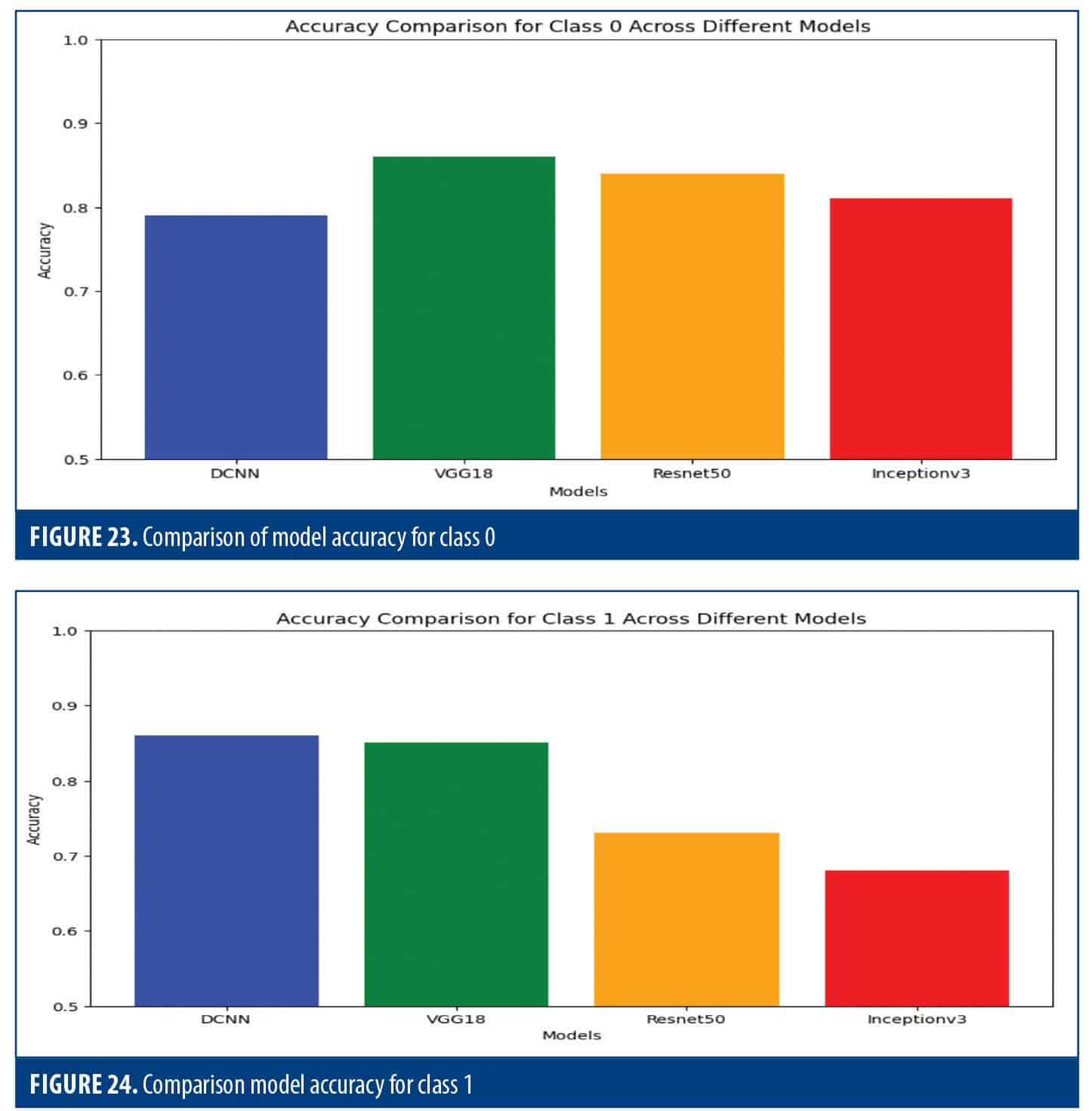
Table 2 dives deeper into the performance of this model for each class, using recall, F1 score, and precision metrics. Class 0 exceled with a precision of 83%, meaning 83% of its classifications for this class were correct. It also achieved a high recall of 86%, indicating it captured 86% of actual class 0 instances. For class 0 the F1 score of 84% demonstrated a great balance between recall and precision. For class 1, the model demonstrated a precision of 77% and a recall of 72%, resulting in an F1 score of 74%. Overall, the model achieved an accuracy of 80%. Macro and weighted F1 scores of 79% and 80%, respectively, suggest uniform performance across the classes.
VGG-16. This model, highly regarded for its balance between clarity and efficiency, is a powerful tool for computer vision tasks. This 16-layer CNN with 138 million parameters leverages several techniques to achieve optimal performance. CT scans were resized and augmented with random flipping, rotation, and brightness variation. This strategy enables the model to learn more robust features and generalize effectively to unseen image. Table 3 showcases VGG-16’s promising improvement over 10 training epochs. Starting with a training loss of 1.15 and validation loss of 0.72, the model steadily reduced training loss to 0.43 by the tenth epoch. This indicates the model was effectively learning from the data. Validation loss follows a similar trend, stabilizing at a low of 0.33. Accuracy reflects this progress, rising from 0.59 to a well-performing 0.86. The error rate correspondingly dropped from 0.41 to 0.14, demonstrating a significant improvement in correct classifications. VGG-16 also excels at identifying specific classes within the data. Recall scores, which measure the model’s ability to capture relevant instances, increased to 0.77. The precision score measures how many of the model’s positive predictions are true positives (TP) in the predictions of the model, was high at 0.85. The F1 score, which balances precision and recall, reached 0.81, confirming the overall effectiveness of the model in classifying classes. Encouragingly, the training time remained consistent throughout the process, averaging 23 to 25 seconds each time.
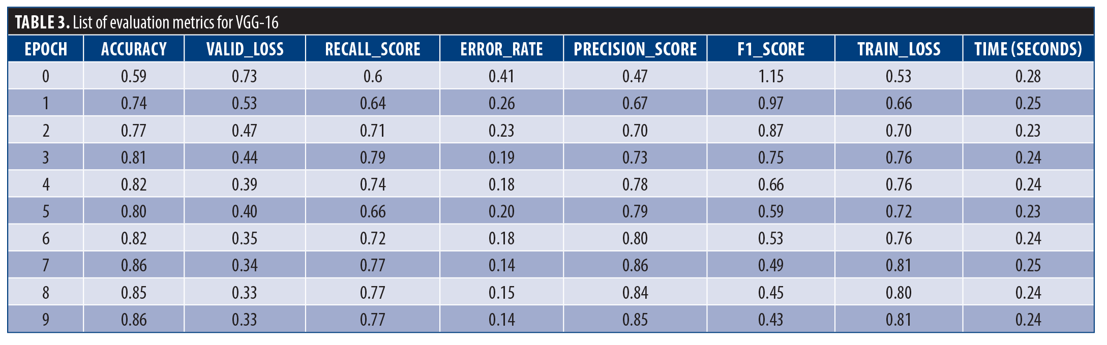
Figure 8 shows the comparison between the predictions of the model and the actual scores for each prediction and the associated loss. It also shows the distribution of predicted probabilities, providing a confidence level contained in its verses. This visualization facilitates the process of evaluating both the accuracy and predictability of the model.
Figure 9 uses the grid structure to display the model predictions along with the ground truth lines of the encounter. This type of visualization provides a quick and efficient way to assess the overall feasibility of a model under various conditions. By analyzing the interaction, we can look at the model’s performance across groups and identify potential strengths or weaknesses. This valuable tool serves 2 purposes: to verify the validity of the model and to identify areas for improvement.
Figure 10 is a confusion matrix that shows the performance of the model on 2 sets of factors as they were divided. There were 138 in class 0, 12 of which were incorrectly identified as class 1 (FP), and 126 correctly identified as class 0 (TN). There were 87 events in class 1; 20 were incorrectly identified as class 0 (FN), while 67 were correctly identified as class 1 (TP). This model did well with class categorization.
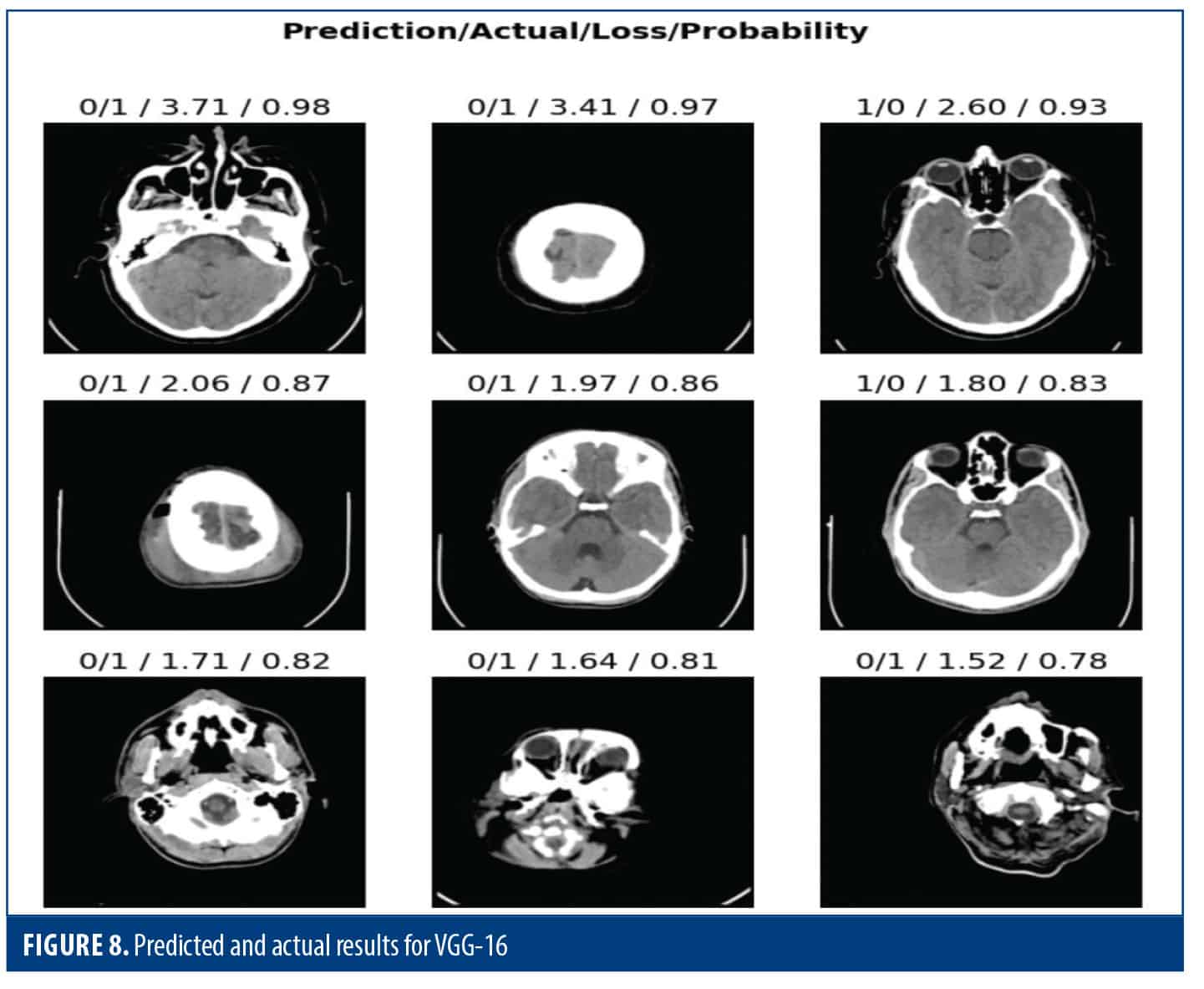
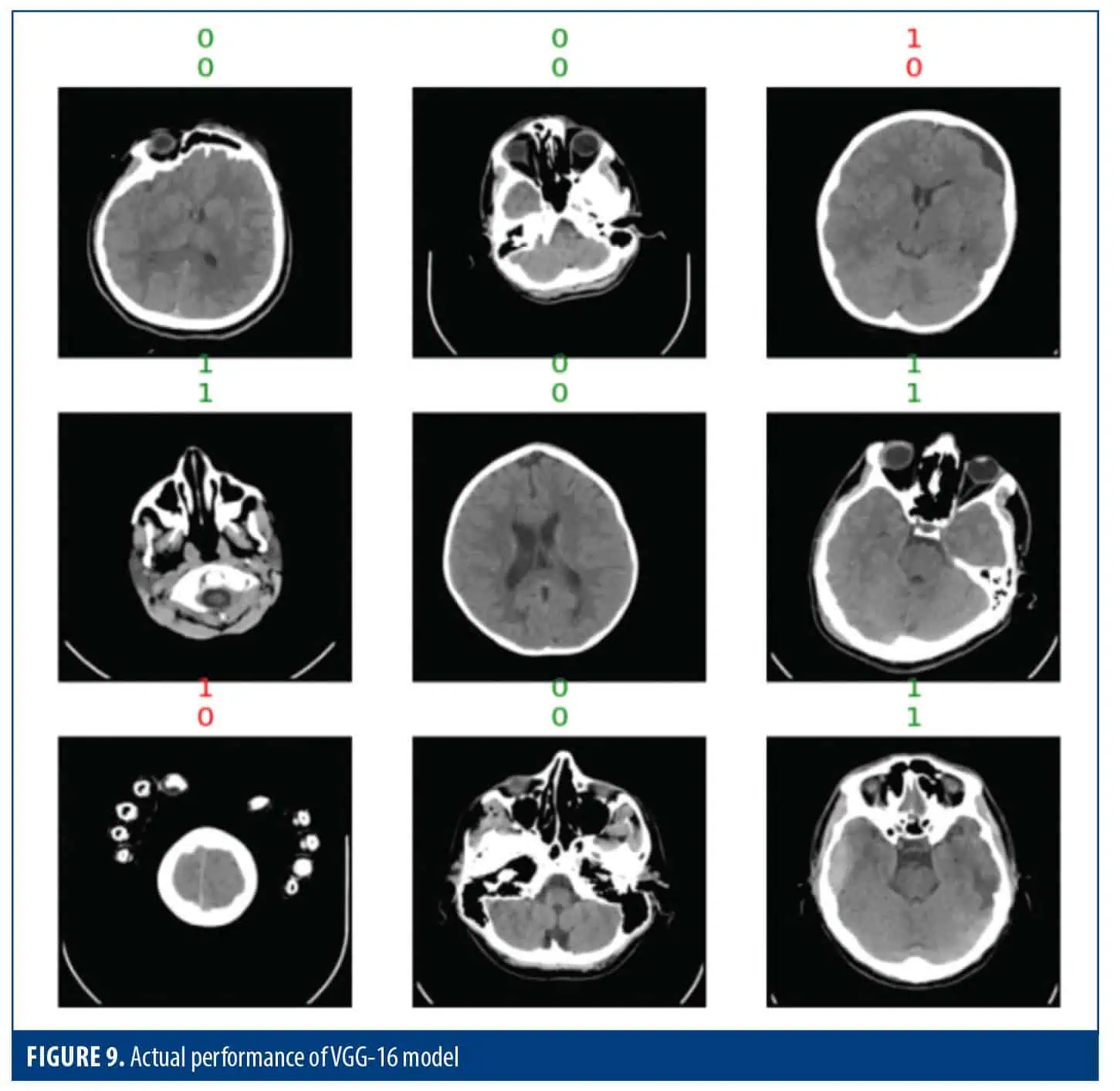
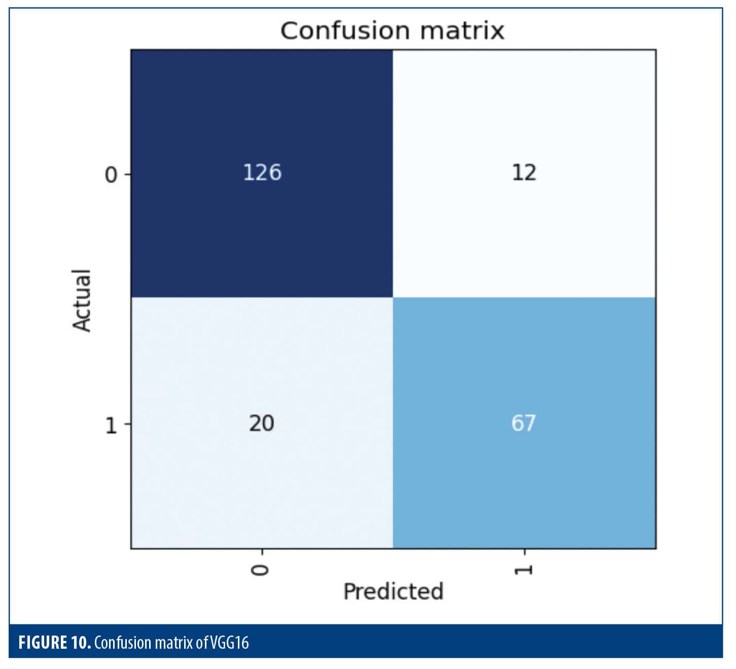
Table 4 shows an in-depth look at how well the model did in 2 different groups. In class 0, the model detected 88% of actual class 0 instances and had a precision of 85%. Only 72% of the actual events were identified for class 1, while accurately predicting 76% of the positive events. The model’s F1 score for both macro and weighted averages was 0.81, and its overall accuracy was 0.82. This suggests that the model’s capacity to categorize cases into these 2 classes is balanced. Class 0 prioritized precision, while class 1 prioritized recall, reflecting a classic trade-off.

ResNet50. This section explores the performance of a ResNet-50 model for image classification tasks. The model leverages several techniques to achieve optimal results (Table 5). Images were resized, and data augmentation techniques were applied. This helps the model learn from a wider variety of image presentations and improve its generalization capability. Over 10 training epochs, the model demonstrated significant improvement. Training loss steadily decreases from 1.25 to 0.37, indicating the model was effectively learning from the data. Notably, validation loss remained stable at a low value of 0.32, suggesting the model was not overfitting. This is further supported by the accuracy rising from 0.70 to a well-performing 0.88, signifying a significant increase in correct classifications. The corresponding error rate decreased from 0.30 to 0.12. The model was also successful in identifying specific classes in the data. The recall score, which reflects the ability of the model to capture context, increased significantly to 0.86. The precision score was high at 0.79. The F1score of 0.83 was decent enough in balancing precision and recall, showing the model’s overall effectiveness in classifying classes. The training time remained consistent at an average of 25 seconds, which is very encouraging.
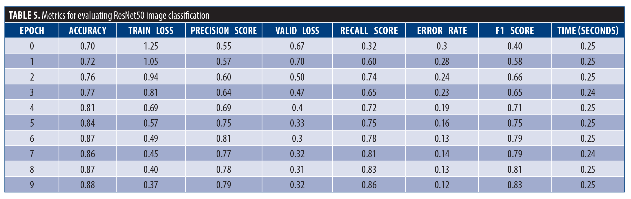
Figure 11 illustrates the outcome obtained by merging the images for a more intricate assessment of the model’s performance. This is where the model predictions are compared against the ground truth scores, and rapid classification accuracy can be assessed. The statistics highlight the problem associated with the prediction and, hence, could be helpful to identify places where the model faces difficulty. Other than that, the probability distribution of the model’s predictions is a representation of the classifier’s confidence in the classification. In general, the overall feature remains a very good indicator to consider in terms of model performance measurement, whether for accuracy or confidence.
Figure 12 illustrates ground truth lines adjacent to model predictions. By analyzing the interaction, we can look at the model’s performance across groups and identify potential strengths or weaknesses. This valuable tool serves two purposes verifying the model’s accuracy and pinpointing areas for improvement.
Figure 13 shows the outcomes of a binary classification task. In total, the model was right about 88.89% of the time, correctly predicting 137 cases of class 0 and 62 cases of class 1. The model worked very well, correctly labeling about 89.55% of the examples that should have been in class 0. It also did a good job with recall. The F1 score was approximately 87.04%, demonstrating the model’s capability of having the proper balance between precision and recall which results in correctly identifying relevant events while controlling for FPs.
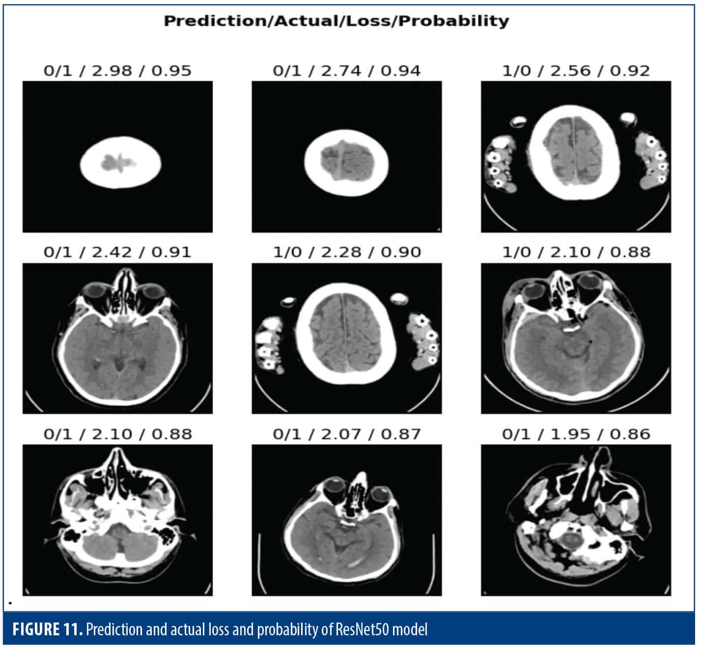
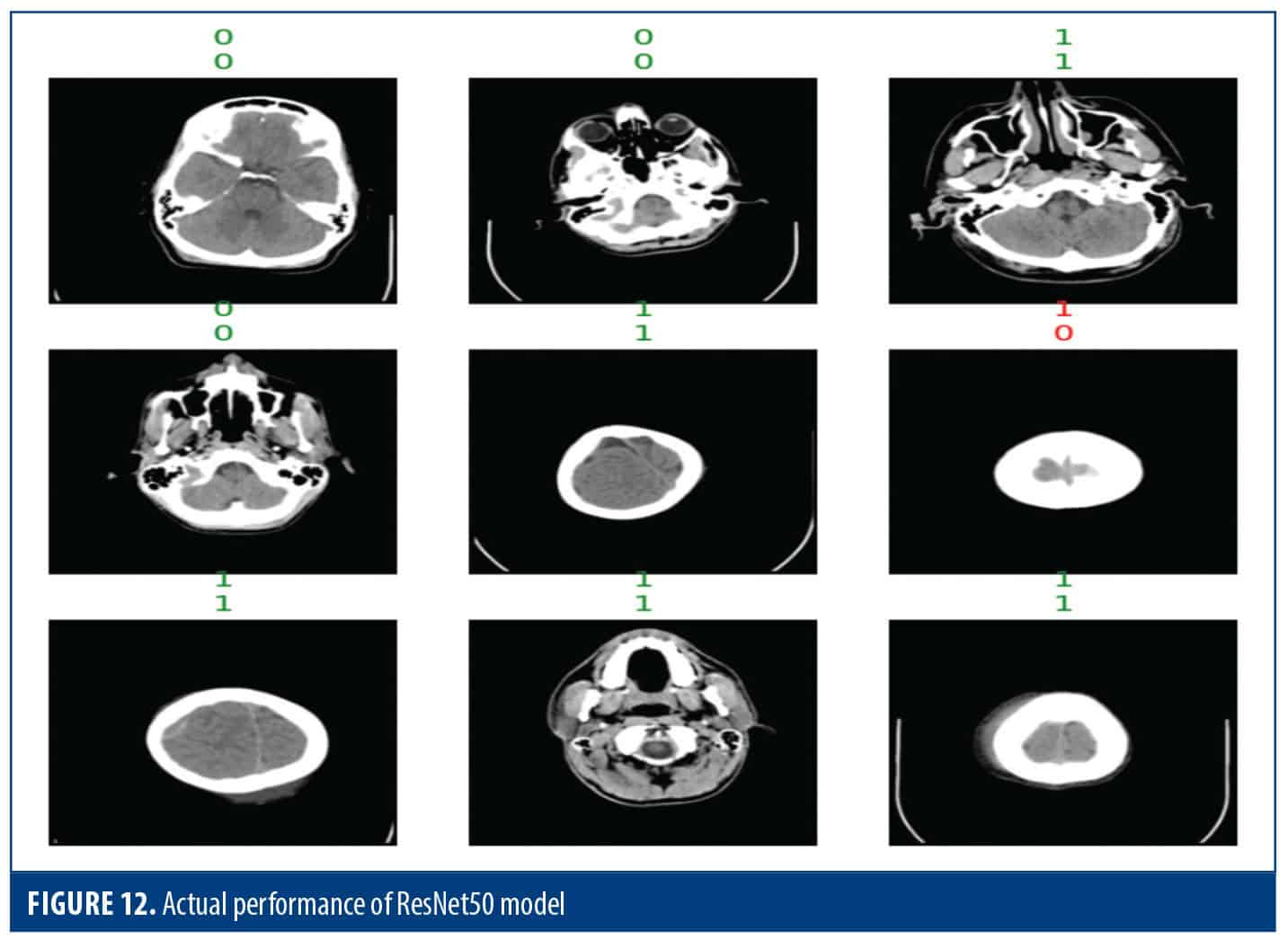
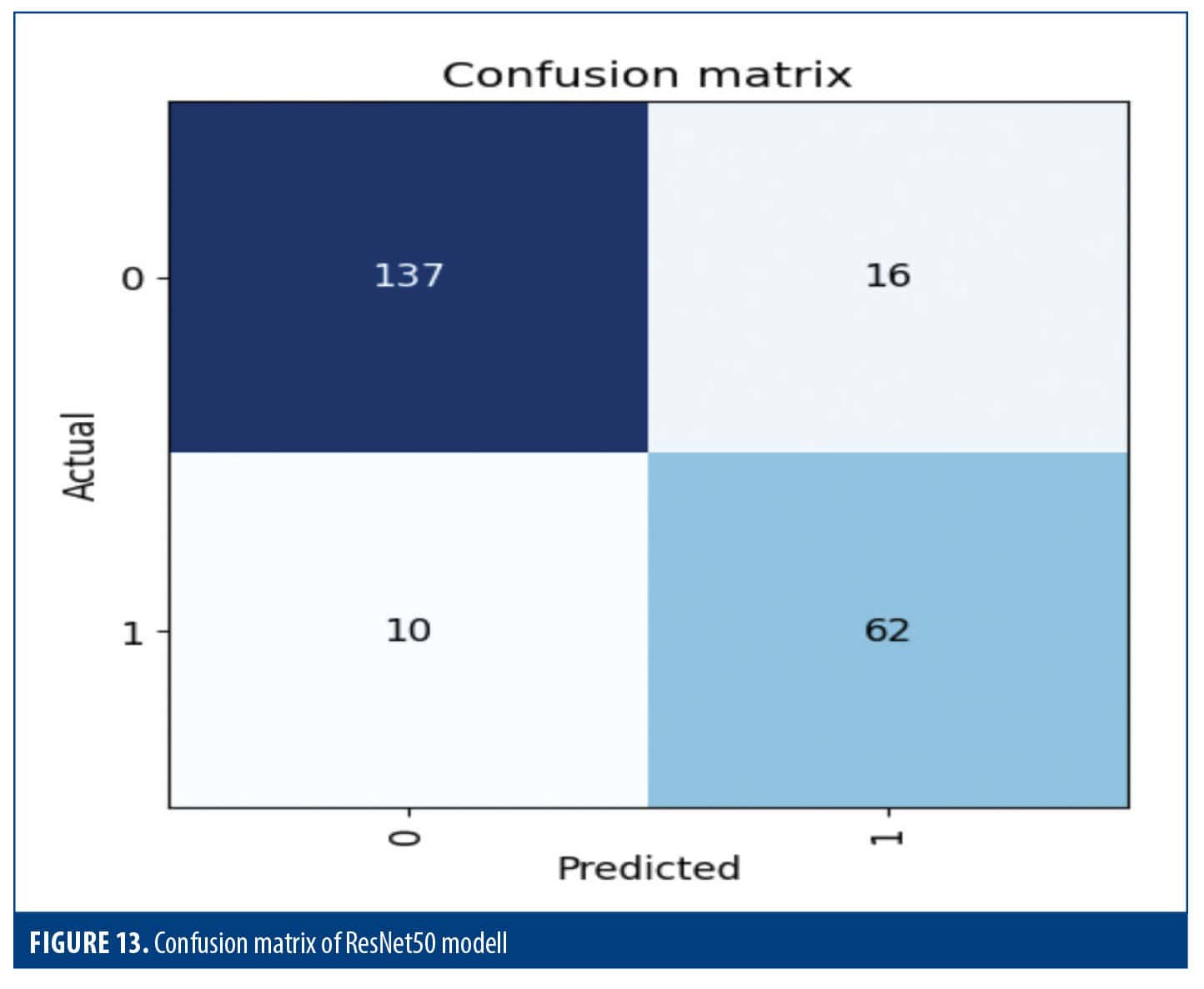
Table 6 shows the classification report which gives an in-depth analysis for the 2 classes, showing that for class 0, the recall (0.92) allowed the model to identify 92% of the true instances while also showing that the accuracy (0.82) was correct only for 82% of the class 0 predictions. The F1score of 0.87 indicates a proper balance of precision and recall. Class 1 had a precision of 0.86, meaning that 86% of predicted instances was correct, and a recall value of 0.73, which means that 73% of actual instances were identified. These scores resulted in an F1 score of 0.83, which indicates that precision and recall performed satisfactorily. Overall, the model ranking on class 0 and class 1 scored an accuracy of 0.80. Macro and weighted averages provide better benchmark scores and help evaluate the balance among classes, particularly in the presence of class imbalance.
Inception v3. All images were resized and data augmentation methods, including flips, rotations, and brightness adjustments, were applied to enhance the diversity of the training dataset. Over the course of 10 training epochs, the model’s training loss decreased steadily, demonstrating its ability to capture underlying patterns. The validation loss remained relatively stable, indicating that the model was not overfitting to the training data. Both accuracy and recall improved as the model progressed, reflecting its enhanced capability to correctly classify images and identify instances within each class. Precision also showed improvement. The F1 score was favorable. Training was computationally efficient, with each epoch completed in approximately 18 to 19 seconds on average (Table 7).
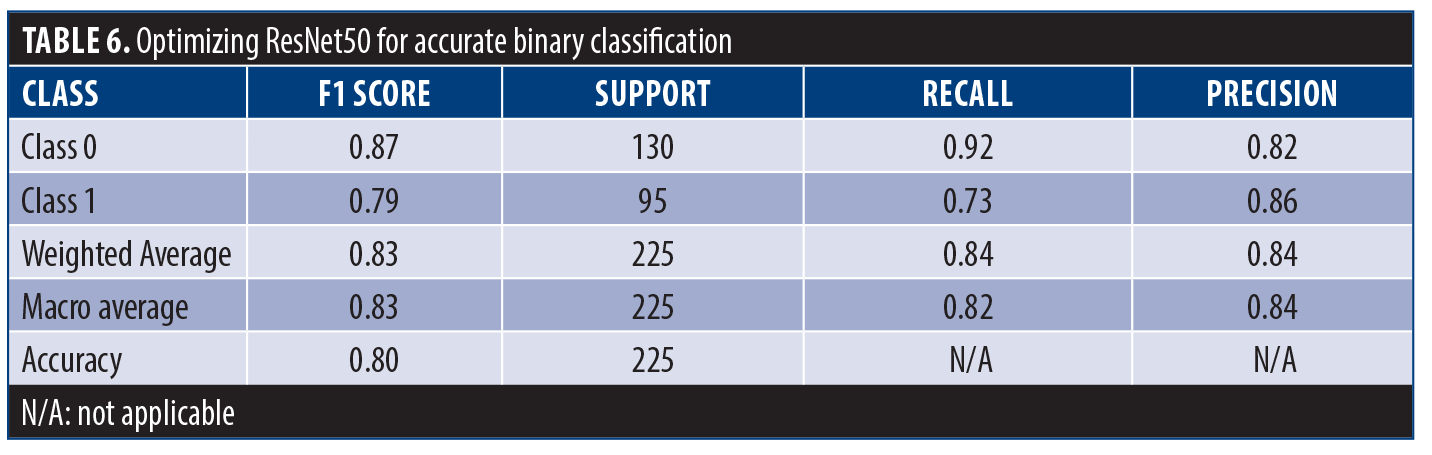
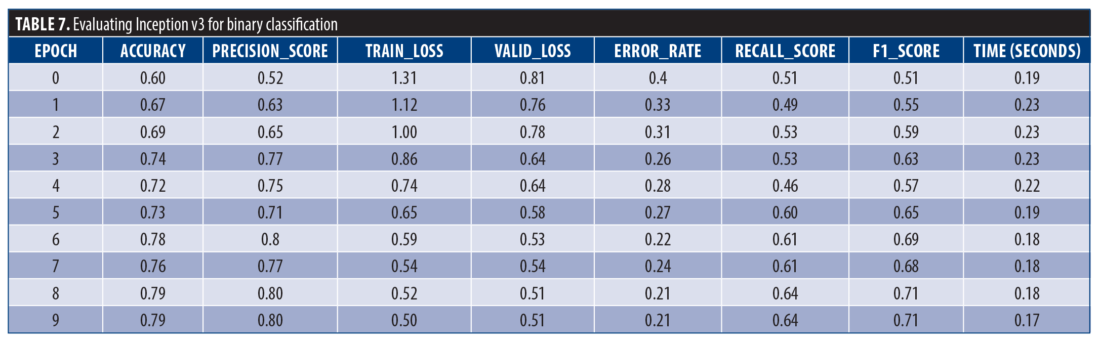
Figure 14 shows how well the model performed in classifying data. In class 0, among 133 actual class 0 instances, the model correctly classified 118 (TNs). However, it mistakenly classified 15 instances as class 1 (FPs). In class 1, the model correctly identified 59 out of 92 actual class 1 instances (TPs) and missed 33 instances by predicting them as class 0 (FNs).
Figure 14 visualizes how the model’s predictions compare to the true labels, revealing both correct classifications and errors. It also shows how confident the model is in each guess (via probabilities) and the severity of its mistakes.
Figure 15 provides displays a grid of images along with what the model predicted (actual label) and what the image truly represents (expected label). This shows how well the model performed across different models and groups. By looking at where the predicted score differs from the expected score, it shows what kind of image the model struggled with and areas for improvement.
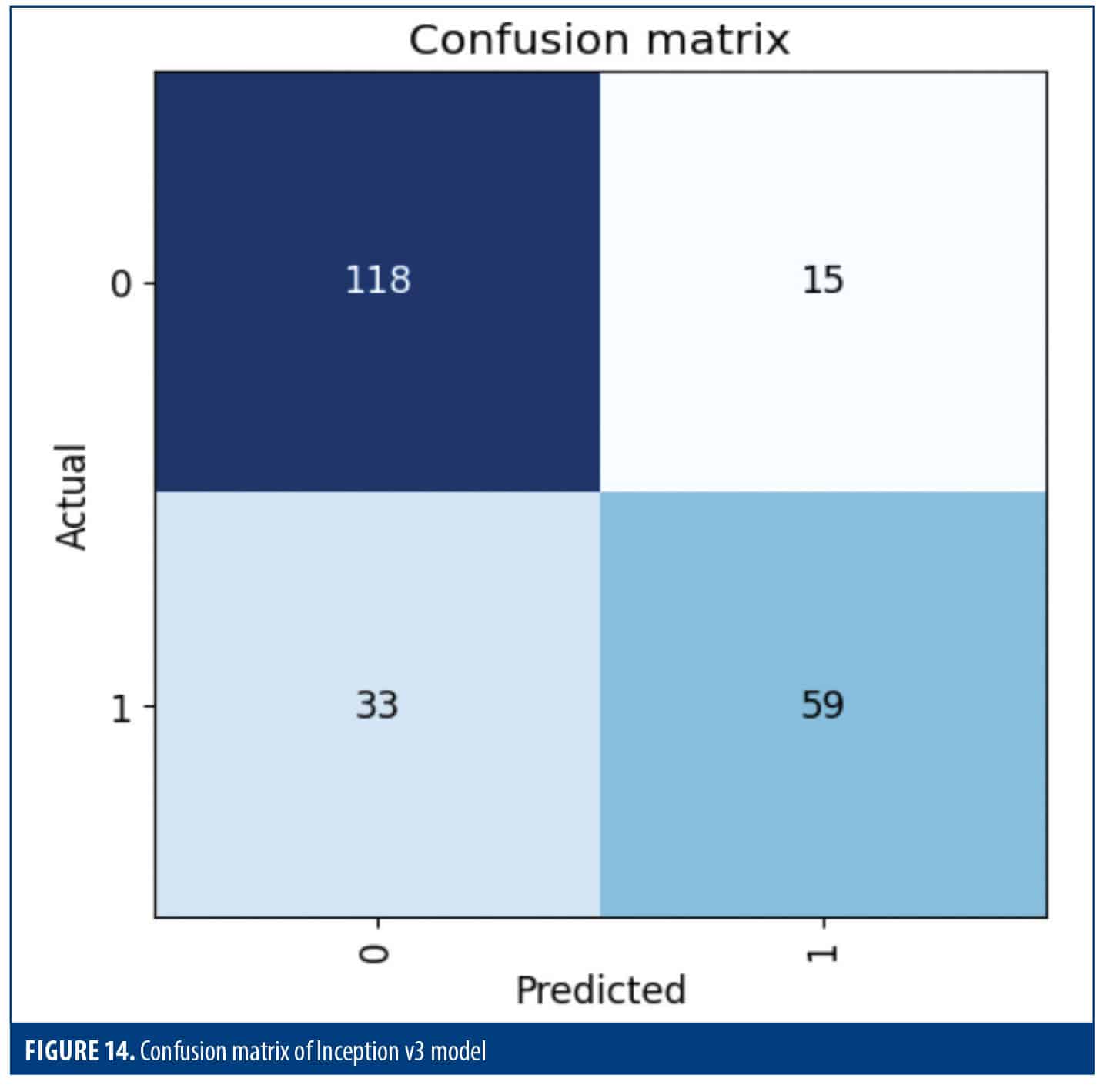
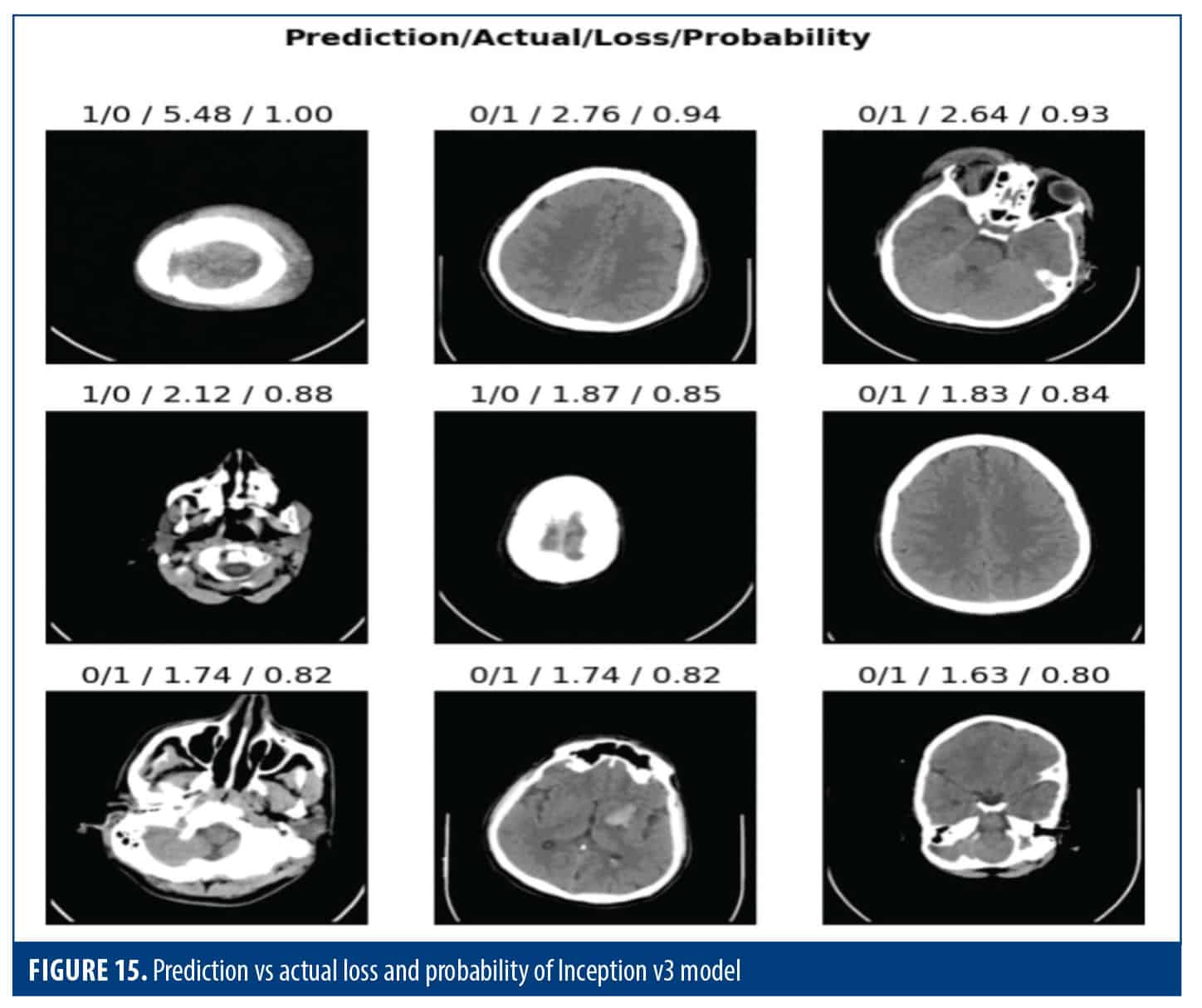
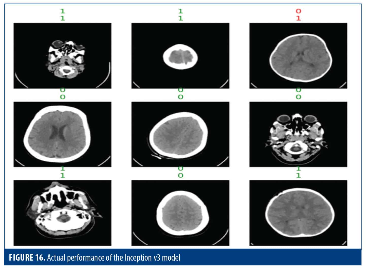
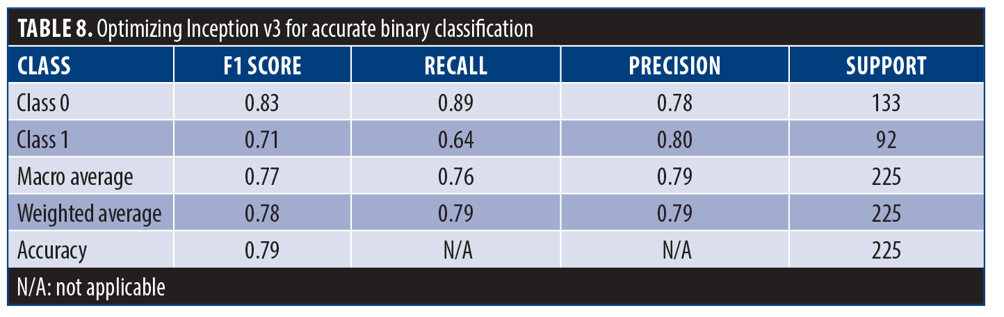
Table 8 involves the performance of the model for each class. It reveals that the model was good at identifying class 0, with high accuracy and recall. However, it did not perform well in class 1, although overall accuracy was still good at 79%, and other metrics, such as the F1 score, show a balanced performance in both classes.
 Discusssion
 Discusssion
This section delves into comparative models using figures and tables. Bar graphs and other charts show how accuracy changes over time, making it easy to see which model performs best. The tables summarize the research parameters, and allow us to look at the strengths and weaknesses of each model in different areas.
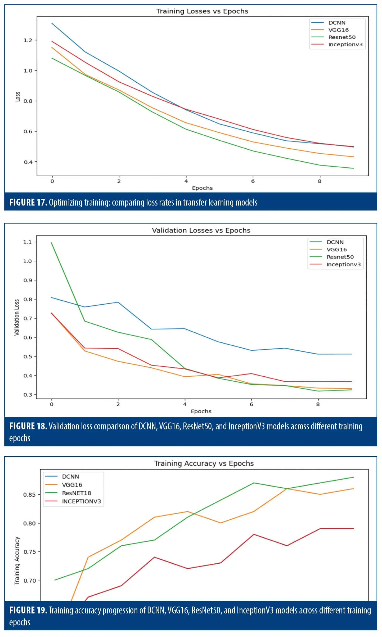
Training loss. All models showed a decreasing trend, indicating successful learning. DCNN stands out with the most consistent decline (Figure 17).
Validation loss. DCNN again showed the most consistent decrease, while VGG-16 and Inception v3 had fluctuations, and ResNet50 started higher before stabilizing (Figure 18).
Training accuracy. VGG-16 consistently achieved the highest training accuracy, followed closely by ResNET50, while DCNN and Inception v3 exhibit comparable but slightly lower accuracy values (Figure 19).
Validation accuracy. DCNN and Inception v3 were consistent. VGG-16 showed improvement, and ResNet50 progressed initially before stabilizing (Figure 20).
Class 0 metrics. DCNN led in precision, recall, and F1 score. VGG-16 and ResNet50 had similar scores (Figure 21).
Class 1 metrics. DCNN outperformed other models, having the highest precision, recall, and F1 score. VGG-16 and ResNet50 had comparable scores (Figure 22).
Class 0 accuracy. VGG-16 had the highest accuracy, followed by ResNet50. Inception v3 and DCNN lagged behind (Figure 23).
Class 1 Accuracy. The DCNN was at the forefront, followed by VGG-16 and ResNet50, while Inception v3 trailed behind (Figure 24).
Implications. Overall, DCNN had the highest average accuracy, followed by VGG-16 and ResNet50 (Table 9). While Inception v3 had balanced metrics, its overall F1 score was slightly lower than the other models. Table 10 highlights the pros and cons of each model, which can aid in choosing the most suitable option for one’s specific needs.
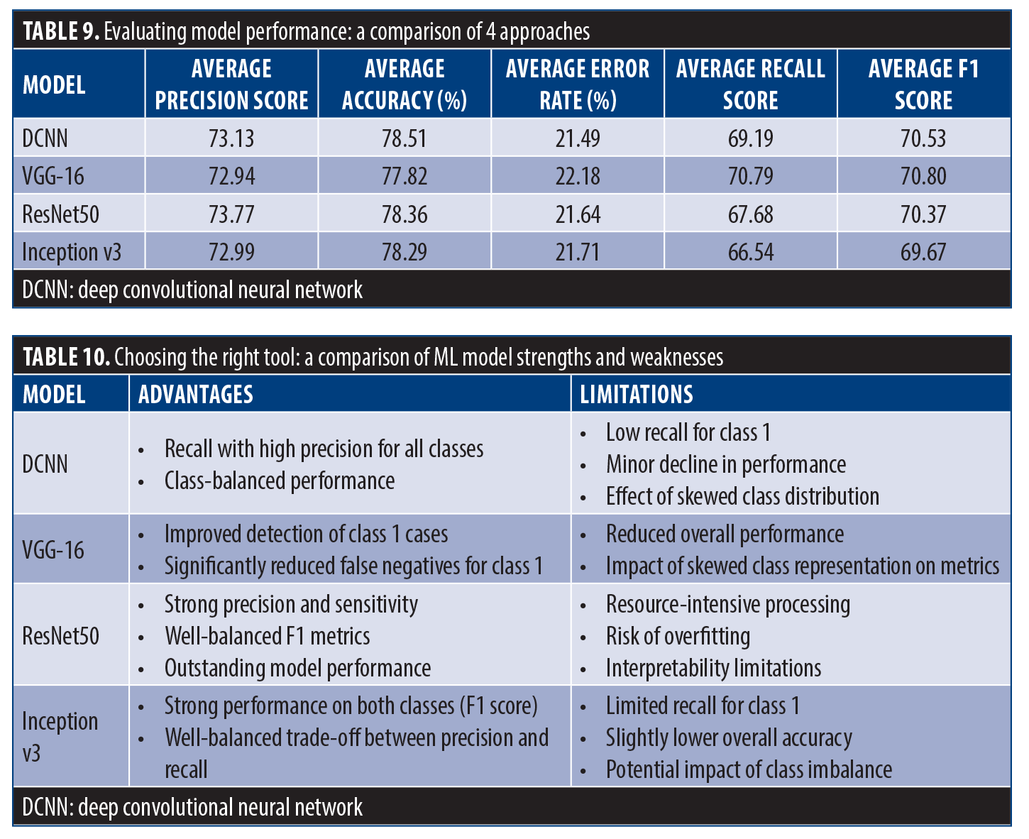
Table 11 shows a comparison of our results with previous studies. Alhatemi et al20 applied a range of deep neural network models (DenseNet121, ResNet50, Xception, MobileNet, VGG-16, and EfficientNetB2) for stroke vs nonstroke MR scan classification using transfer learning. The study datasets contained 1,901 training images, 475 validation images, and 250 test images, with data augmentation employed to enhance learning of the DL model. Advanced EfficientNetB2 model produced the best outcome, with overall accuracy, precision, recall, and F1 score at 98.8%, thereby demonstrating state-of-the-art performance compared with previously reported methods on the same dataset. As an alternative, Lo et al50 focused on building an automation system for the detection of acute ischemic stroke utilizing DCNN using NCCT images with a total of 1,254 grayscale NCCT images obtained from 96 patients and 121 healthy controls with high accuracy, sensitivity, and specificity. They found model accuracy when trained from scratch to be at least equivalent to, if not better than, a transfer learning–trained model, but it did have hints of a genuine domain quality for acute ischemic stroke diagnosis, for use with specific scanners. Abboui et al51 conducted a detailed study of DL models for accurate cerebral ischemic stroke classification using Moroccan medical data. The VGG-16 framework was implemented using transfer learning, and data enhancement techniques were used to improve the performance of the model. The developed model outperformed other state-of-the-art models in terms of validation accuracy, including ResNet50 (87.0%), Inception v3 (82.0%), VGG-19 (81.0%) and achieved an impressive validation accuracy of 90%.
Comparing our research findings with existing studies on ischemic stroke classification using CT scans, we have demonstrated superior accuracy rates across multiple models. Our results outperform previous studies, with our DCNN model achieving an accuracy of 79.0%, VGG-16 at 86.0%, ResNet50 at 88.0%, and Inception v3 at 79.0%. Additionally, our approach boasts faster processing times, with respective average times of 19, 24, 25, and 20 seconds, further underscoring the efficacy of our methodology in stroke diagnosis. Although prior studies boast high accuracy and good performance indices, they do not consider the issue of time. In our study, we not only obtained high accuracy, but also stressed the importance of timely diagnosis by incorporating the fastai study and emphasizing it in-depth. This integration allowed us to evaluate the computational effort and execution time of the models, ensuring that they can be successfully applied in clinical settings. Furthermore, we provided a comprehensive analysis of class 0 (normal) and class 1 (stroke) results for each case to analyze the models under different conditions. In addition to providing helpful insights, we provided visual results, increasing the interpretation and clarity of our findings, which is critical to gaining trust and acceptance by the medical profession. Overall, our study aims to bridge the gap between the efficacy of DL models for diagnosis during traumatic brain injury and their practical utility. It should also be recognized that lesion visibility on NCCT is not absolute but context-dependent. Factors such as lesion size, depth, and vascular territory play a major role in detectability, and small or early infarcts may remain inconspicuous. Moreover, lesion cause and accompanying clinical information, when integrated with neuroanatomical hypotheses, significantly enhance diagnostic certainty. Our proposed approach should therefore be viewed as a complementary tool that augments, rather than replaces, the neuroanatomical reasoning applied by clinicians.
Limitations. One limitation of our study is that we relied on existing datasets rather than an original dataset, which may introduce bias. In addition, our focus on 1 modality, CT scan, may limit the generalizability of our findings. Combining other methods and performing real-time validation in clinical settings could increase the practical applicability and accuracy of our model. Another limitation of this study is the lack of standardized information regarding the time of NCCT acquisition relative to stroke onset. Since lesion detectability on CT is strongly time-dependent, with early ischemic changes often being subtle and late changes more conspicuous, the inclusion of scans from different temporal stages may have affected both ground truth labeling and model performance. Future work should focus on datasets with well-documented imaging timelines to better capture the dynamic evolution of ischemic lesions.
Conclusions and future directions
This research explored how DL models could be used to classify brain strokes using CT scans. To speed up training and enhance model performance, we employed transfer learning, a method that leverages pretrained models that trained on large image datasets. Various pretrained CNN architectures, such as ResNet, VGG, Inception, and EfficientNet, were fine-tuned using a dataset of CT scans labeled for normal and stroke-affected brains. The fastai library was crucial in facilitating the training process and potentially reducing training times. We evaluated model performance using several metrics, including accuracy, precision_score, train_loss, valid_loss, error_rate, recall_score, f1_score, and time, both in training and testing cases. Through iterative adjustments and rigorous evaluation, ResNet50 emerged as the most accurate model, achieving an impressive 88% accuracy in identifying stroke presence in CT scans. Additionally, we found that the DCNN model took the least amount of time for training. These findings underscore the promise of DL techniques, particularly when coupled with transfer learning and the fastai library. By harnessing pretrained models and optimizing training procedures, DL holds the potential to enable quicker and more accurate patient categorization based on CT scans. This advancement could significantly enhance patient outcomes by facilitating timely and precise diagnosis, leading to more effective stroke treatment strategies.
Still, there are a number of ways that more study and development could be done. To begin, making more detailed changes to the hyperparameters might make the models work better, especially for brain stroke cases. Additionally, looking into the use of ensemble methods—for example, combining best features from several models—might lead to better results. We might get a better understanding of how the models make decisions with the use of other modalities, such as MRI and angiography. Also, collecting and using larger, more varied datasets might make it easier to check how well the models work in more situations. Finally, conducting user studies and putting these models to use in real-world situations could show that they work in such settings.
Availability of dataset
We got the data used for this study from the publicly available dataset Brain Stroke CT Image Dataset on Kaggle, a popular data science and ML platform. CT images were sourced from a number of medical institutions. We used the CT images in this study for detection of brain stroke.
References
- Sirsat MS, Fermé E, Camara J. Machine learning for brain stroke: a review. J Stroke Cerebrovasc Dis. 2020;29(10):105162.
- Kuo W, Häne C, Mukherjee P, et al. Expert-level detection of acute intracranial hemorrhage on head computed tomography using deep learning. Proc Natl Acad Sci USA. 2019;116(45):22737–22745.
- Chin CL, Lin BJ, Wu GR, et al. An automated early ischemic stroke detection system using CNN deep learning algorithm. 2017 IEEE 8th International Conference on Awareness Science and Technology (iCAST). 2017;368–372.
- Khan P, Kader MF, Islam SR, et al. Machine learning and deep learning approaches for brain disease diagnosis: principles and recent advances. IEEE Access. 2021;9:37622–37655.
- Dourado CM, da Silva SPP, da Nobrega RVM, et al. An open IoHT-based deep learning framework for online medical image recognition. IEEE J Sel Areas Commun. 2020;39(2):541–548.
- Gao XW, Hui R, Tian Z. Classification of CT brain images based on deep learning networks. Comput Methods Programs Biomed. 2017;138:49–56.
- Chowdhary CL, Acharjya DP. Segmentation and feature extraction in medical imaging: a systematic review. Procedia Computer Science. 2020;167:26–36.
- Zhang S, Wang J, Pei L, et al. Interpretable CNN for ischemic stroke subtype classification with active model adaptation. BMC Med Inform Decis Mak. 2022;5;22(1):3.
- Gautam A, Raman B. Towards effective classification of brain hemorrhagic and ischemic stroke using CNN. Biomedical Signal Processing and Control. 2021;63:102178.
- Li L, Wei M, Liu B, et al. Deep learning for hemorrhagic lesion detection and segmentation on brain CT images. IEEE J Biomed Health Inform. 2021;25(5):
1646–1659. - Liu T, Fan W, Wu C. A hybrid machine learning approach to cerebral stroke prediction based on an imbalanced medical dataset. Artif Intell Med. 2019;101:101723.
- Goldstein LB, Jones MR, Matchar DB, et al. Improving the reliability of stroke subgroup classification using the Trial of ORG 10172 in Acute Stroke Treatment (TOAST) criteria. Stroke. 2001;32(5):1091–1098.
- Sung SF, Lin CY, Hu YH. EMR-based phenotyping of ischemic stroke using supervised machine learning and text mining techniques. IEEE J Biomed Health Inform. 2020;24(10):2922–2931.
- Govindarajan P, Soundarapandian RK, Gandomi AH, et al. Classification of stroke disease using machine learning algorithms. Neural Computing and Applications. 2020;32:817–828.
- Walsh KB. Non-invasive sensor technology for prehospital stroke diagnosis: Current status and future directions. Int J Stroke. 2019;14(6):592–602.
- Salucci M, Polo A, Vrba J. Multi-step learning-by-examples strategy for real-time brain stroke microwave scattering data inversion. Electronics. 2021;10(1):95.
- Bajaj S, Bala M, Angurala M. Machine learning models for enhanced stroke detection and prediction. Egypt Inform J. 2025;30:100705.
- Nielsen MA. Neural Networks and Deep Learning. Determination Press; 2015.
- Pedregosa F, Varoquaux G, Gramfort A, et al. Scikit-learn: machine learning in Python. J Mach Learn Res. 2011;12:2825–2830.
- Alhatemi RAJ, Savaş S. Transfer learning-based classification comparison of stroke. JCS. 2022;IDAP-2022: International Artificial Intelligence and Data Processing Symposium:192–201.
- Howard J, Gugger S. Fastai: a layered API for deep learning. Information. 2020;11(2):108.
- Raj R, Mathew J, Kannath SK, Rajan J. StrokeViT with AutoML for brain stroke classification. Eng Appl Artif Intell. 2023;119:105772.
- Karthik R, Menaka R, Johnson A, Anand S. Neuroimaging and deep learning for brain stroke detection – a review of recent advancements and future prospects. Comp Methods Programs Biomed. 2020;197:105728.
- Amin R, Al Ghamdi MA, Almotiri SH, Alruily M. Healthcare techniques through deep learning: issues, challenges, and opportunities. IEEE Access. 2021;9:98523–98541.
- Dourado CM, da Silva SPP, da Nobrega RVM, et al. Deep learning IoT system for online stroke detection in skull computed tomography images.Comput Netw. 2019; 152:25–39.
- Karthik R, Gupta U, Jha A, et al. A deep supervised approach for ischemic lesion segmentation from multimodal MRI using fully convolutional network. Applied Soft Computing. 2019;84:105685.
- He K, Zhang X, Ren S, Sun J. Deep residual learning for image recognition. Proceedings of the IEEE Conference on Computer Vision and Pattern Recognition. 2016;770–778.
- Howard AG, Zhu M, Chen B, Kalenichenko D, Wang W, et al. Mobilenets: efficient convolutional neural networks for mobile vision applications. arXiv preprint. 2017;arXiv:1704.04861.
- Simonyan K, Zisserman A. Very deep convolutional networks for large-scale image recognition. arXiv preprint. 2014;arXiv:1409.1556.
- Savaş S, Topaloğlu N, Kazcı Ö, Koşar P. Comparison of deep learning models in carotid artery Intima-Media thickness ultrasound images: CAIMTUSNet. Bilişim Teknolojileri Dergisi. 2022;15(1):1–12.
- Huang G, Liu Z, Van Der Maaten L, Weinberger KQ. Densely connected convolutional networks. Proceedings of the IEEE Conference on Computer Vision and Pattern Recognition. 2017;4700–4708.
- Chollet F. Xception: deep learning with depthwise separable convolutions. Proceedings of the IEEE Conference on Computer Vision and Pattern Recognition. 2017;1251–1258.
- Szegedy C, Vanhoucke V, Ioffe S, Shlens J, Wojna Z. Rethinking the inception architecture for computer vision. Proceedings of the IEEE Conference on Computer Vision and Pattern Recognition. 2016;2818–2826.
- Kingma DP, Ba J, Bengio Y, LeCun Y. ADAM: a method for stochastic optimization. arXiv preprint. 2017;arXiv:1412.6980.
- Salau AO, Jain S. Feature extraction: a survey of the types, techniques, applications. 2019 International Conference on Signal Processing and Communication (ICSC). 2019;158–164.
- Fan J, Chen M, Luo J, et al. The prediction of asymptomatic carotid atherosclerosis with electronic health records: a comparative study of six machine learning models. BMC Med Inform Decis Mak. 2021;21:115.
- Ortiz-Ramón R, Hernández MDCV, González-Castro V, et al. Identification of the presence of ischaemic stroke lesions by means of texture analysis on brain magnetic resonance images. Comput Med Imaging Graph. 2019;74:12–24.
- Han SW, Kim SH, Lee JY, et al. A new subtype classification of ischemic stroke based on treatment and etiologic mechanism. Eur Neurol. 2007;57(2):96–102.
- Orr GB, Müller KR, eds. Neural Networks: Tricks of the Trade. Springer Berlin Heidelberg; 1998.
- Wang G, Ye JC, Mueller K, Fessler JA. Image reconstruction is a new frontier of machine learning. IEEE Trans Med Imaging. 2018;37(6):1289-1296.
- Draelos RL, Carin L. Use HiResCAM instead of Grad-CAM for faithful explanations of convolutional neural networks. arXiv preprint. 2020;arXiv:2011.08891.
- Magadza T, Viriri S. Deep learning for brain tumor segmentation: a survey of state-of-the-art. J Imaging. 2021;7(2):19.
- Folego G, Weiler M, Casseb RF, et al. Alzheimer’s disease detection through whole-brain 3D-CNN MRI. Front Bioeng Biotechnol. 2020;8:534592.
- Haller S, Van Cauter S, Federau C, et al. The R-AI-DIOLOGY checklist: a practical checklist for evaluation of artificial intelligence tools in clinical neuroradiology. Neuroradiology. 2022;64(5):851–864.
- Mei X, Liu Z, Robson PM, et al. RadImageNet: an open radiologic deep learning research dataset for effective transfer learning. Radiol Artif Intell. 2022;4(5):e210315.
- Bajaj S, Bala M, Angurala M. A comparative analysis of different augmentations for brain images. Med Biol Eng Comp. 2024;62(10):3123–3150.
- Wang D, Han C, Zhang Z, et al. FedDUS: lung tumor segmentation on CT images through federated semi-supervised with dynamic update strategy. Comput Methods Programs Biomed. 2024;249:108141.
- Pérez-Velasco S, Marcos-Martínez D, Santamaría-Vázquez E, et al. Unraveling motor imagery brain patterns using explainable artificial intelligence based on Shapley values. Comput Methods Programs Biomed. 2024;246:108048.
- Farkhani S, Demnitz N, Boraxbekk CJ, et al. End-to-end volumetric segmentation of white matter hyperintensities using deep learning. Comput Methods Programs Biomed. 2024;245:108008.
- Lo CM, Hung PH, Lin DT. Rapid assessment of acute ischemic stroke by computed tomography using deep convolutional neural networks. J Digit Imaging. 2021;34(3):
637–646.
- Abbaoui W, Retal S, Ziti S, El Bhiri B, Moussif H. Ischemic stroke classification using VGG-16 convolutional neural networks: a study on Moroccan MRI scans. Int J Online Biomed Eng. 2024;20(2):61–77.